Developing and Implementing Scenario Analysis Models to Measure Operational Risk at Intesa Sanpaolo

In 1995, Barings Bank went bankrupt following a $1.4 billion loss due to unauthorized trading activity. Ten years later, JP Morgan agreed to pay a $2.2 billion settlement after the Enron scandal. More recently, Société Générale suffered a €4.9 billion loss following multiple breaches of control in its trading activities.

Events like these highlight the enormous economic impact of operational risk—defined in the new Basel Accord (Basel II) as “the risk of loss resulting from inadequate or failed internal processes, people, and systems or from external events.” Basel II requires financial institutions to hold capital against unexpected losses arising from operational risk.

At Intesa Sanpaolo, we used MATLAB to build entirely new scenario analysis models that enable compliance with Basel II requirements. Scenario analysis is a key component of the advanced measurement approach (AMA) to estimating the capital charge for operational risk. Introduced in Basel II, AMA imposes strict quantitative requirements for measuring operational risk. For example, it requires the calculation of a capital measure to the 99.9% confidence level over a one-year holding period.

MATLAB saved us a significant amount of prototyping and development time. It also gave us flexibility­—particularly useful in the early trial-and-error stages of the project, when we often made substantial changes to test new ideas.

Implementing Scenario Analysis

Unlike traditional techniques, scenario analysis uses expert opinion as input rather than historical data. Given the vast scope of scenario analysis at Intesa Sanpaolo (it encompasses all departments of the bank), gathering expert opinion via face-to-face interviews was simply not possible. For efficiency, therefore, we used questionnaires.

The main technical challenges in developing a scenario analysis framework and tools were determining which kind of sensitivity to extreme loss outcome the interviewees would be able to report. We needed a process and a model that could “guide” the experts but leave them final responsibility for their estimates. This translated into a huge numerical calibration effort during model development, involving for example, creating meaningful ranges for estimates.

Recognizing that operational risk is often associated with extraordinary events, Intesa Sanpaolo has adopted a Value-at-Risk (VaR) approach to operational risk measurement. The adoption of VaR required us to find a suitable distribution and to use a robust calibration analysis for data modeling and extrapolation. Thorough calibration is required because VaR is a tail risk measure that deals with often “unobserved” risk scenarios. For example, estimating the risk of a financial scandal such as Enron requires extrapolation, because the final outcome is well beyond the range of observed data. As such, modeling choices can produce vastly different results.

The design and fine-tuning of the scenario analysis model required two capabilities supported by MATLAB: sophisticated sensitivity analysis and the collection and graphical exploration of analysis results. Given the problem’s scope and complexity—hundreds of loss distributions must be considered jointly—the analysis can be a significant challenge.

We divided the model-development process into four steps: developing the basic algorithm, calibrating the model input, setting up ranges in risk assessment questionnaires, and estimating capital at risk.

Developing the Basic Algorithm

Our scenario analysis (SA) algorithm is based on the loss distribution approach (LDA). LDA is standard in the insurance field, which deals with the same types of challenges as those inherent in operational risk. Because we calculate the yearly loss distribution in terms of its frequency and severity, the key information was the expected annual frequency of loss events (used to calibrate the frequency distribution) and the economic impact of each event (used to calibrate the severity distribution). We input the frequency and severity components separately. This allowed the expert assessor to answer the questionnaire in terms of frequency and severity and produced both qualitative and quantitative information.

The SA algorithm inputs the questionnaire responses, which we use to calibrate the frequency and severity distributions. Poisson and negative binomial distributions are both suitable for modeling the frequency distributions of operational losses. We chose Poisson to model the frequency distributions because it is a single-parameter discrete distribution commonly used for insurance and aggregate risk modeling. For the severity distribution, we selected Lognormal.

We used MATLAB and the lognrnd() function from Statistics and Machine Learning Toolbox™ to estimate the 99.9% VaR of the aggregate loss distribution. Our MATLAB code uses a Monte Carlo method, as follows:

%% data
dim=1e6; % number of scenarios
mu=9;sigma=2;   % severity (lognormal)      
                % parameters
lambda=100;     % frequency parameter 
        % (average frequency)
%% Monte Carlo using cellfun 
N=num2cell(poissrnd(lambda,dim,1)); 
Loss = cellfun(@(x) sum(lognrnd...
(mu,sigma,x,1)), N,... 
'UniformOutput', false); 
Loss=cell2mat(Loss);   
   % aggregate loss 
   % distribution (empirical)
VaR=prctile(Loss,99.9);

Note that cellfun enabled us to avoid loops and write very compact code.

Calibrating the Model Input

A critical issue for scenario analysis is the quality of model input. The key information required for each risk class is the expected annual frequency (λ) of the loss events and the economic impact of each event, evaluated in terms of typical loss (M) and worst case (WC) scenario. We calibrate the frequency distribution using λ and calibrate the severity distribution using M and WC.

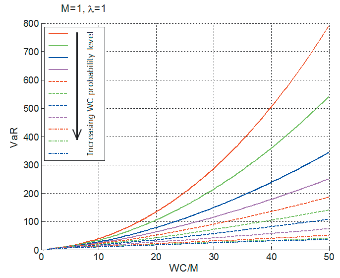
Because WC is the most important parameter for determining capital at risk, we made sure that we had the correct interpretation for this parameter. Figure 1 shows the results of our sensitivity analysis for WC calibration.

For example, suppose that the solid red line represents a probability level of 98% and the dashed red line represents 99%. If an assessor answered with a typical loss of 1 and a worst case of 30 (M=1, WC=30), then WC/M would be 30 and we would obtain a VaR equal to 300 in the first case and 100 in the second. In other words, if the model interprets WC as the 98% quantile of severity distribution rather than 99%, we obtain a VaR that is three times higher.

There are many ways to interpret WC, including a fixed (high) quantile of severity distribution, worst single loss in a fixed period, and a quantile of severity distribution with a probability level that depends on average frequency. The latter approach combines a probabilistic with a scenario analysis approach. We conducted a similar analysis for the interpretation of the typical loss, M.

Setting up Ranges in Risk Assessment Questionnaires

Because our experts must estimate some metrics, we asked them to express their answers as ranges rather than as point estimates. Our goal was to ensure consistency and efficiency while preserving the features that were specific to business units (for example, size and business activity).

The homogeneity property of linear systems. enabled us to simplify our reasoning by operating in a “normalized” world: We could calculate just once (and in advance) a “normalized VaR”—that is, one computed for a typical loss of 1. To save time, we calculated a normalized VaR as a function of only the WC/M ratio and the frequency.

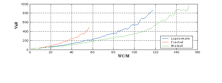
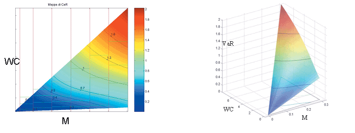
Figure 2 shows the results of simulations carried out on three different severity distributions. Figure 3 shows VaR as a function of M and WC.

We found that we could scale the results by simply multiplying by the relevant typical loss, M. Once we had set normalized ranges of estimates, we could scale them using this business-unit-specific indicator. By checking and balancing the outcome variance in each class, we optimized the setting of ranges.

Estimating Capital at Risk

To aggregate the questionnaire answers to estimate the group-level VaR, we applied the basic LDA algorithm to every answer and then aggregated all the answers, taking into account the effects of diversification.

To induce a target, linear or rank correlation, we used a restricted pairing algorithm, which is similar to a Gaussian copula. The approach we implemented, a refinement of the Iman-Conover method (1982), allows for a closer match between target and resulting correlation matrix.

Putting the Model to Work

Putting all these steps together, we developed an automated tool that performs the necessary statistical computations and automatically generates reports in Excel and PowerPoint. We are now finalizing the first version of the AMA model to be used for regulatory capital purposes.

Operational risk managers are currently using the tool to manage the entire scenario analysis calculation process from setting up answer ranges to estimating the group-level VaR.

The model that we developed can be used in any application that involves collecting expert opinion and turning it into numerical estimates—for example, it can be used in the insurance industry to measure solvency risk in insurance, and in the energy industry to forecast gas consumption or conduct risk analysis connected to oil exploration and production. It is easy to incorporate insurance coverage into the model and use Monte Carlo simulation to estimate its mitigation effect. Used in this way, scenario analysis can be a useful tool for estimating the effectiveness of insurance policies and for optimizing policy limits and deductibles in a cost-benefit analysis.

Our scenario analysis model satisfies the requirements of Basel II because it estimates capital measure at the 99.9% confidence level over a one-year holding period. Implementing the model does not automatically satisfy Basel II requirements; before it can be used for official work, it is subject to thorough review by financial regulators. This is key point to remember as you design and develop a scenario analysis framework.

Statements in this article are intended as the exclusive opinions of the authors and do not necessarily represent those of Intesa Sanpaolo Group. This article was completed while Andrea Colombo was with Intesa Sanpaolo.