An Experiment in Deep Learning with Wild Animal Trail Camera Data
By Cleve Moler, MathWorks
Trail cameras are automatically triggered by animal movements. They are used by ecologists and wildlife managers around the world to study wild animal behavior and help preserve endangered species. I want to see if MATLAB® image processing and deep learning can be used to identify individual animal species that visit trail cameras. We are going to start with off-the-shelf functionality—nothing specialized for this particular task.
My partners on this project are Heather Gorr and Jim Sanderson. Heather is a machine learning expert at MathWorks. Jim was one of my Ph.D. students at the University of New Mexico. He spent several years at Los Alamos National Laboratory writing Fortran programs for supercomputers. But an interest in nature photography evolved into a desire to switch to a career in ecology. He is now the world’s leading authority on small wild cats. He is also the proprietor of CameraSweet, a software package used by investigators around the world to classify and analyze their trail camera data.
Our Data
Our study uses data collected by the United States Fish and Wildlife Service (FWS) office in Albuquerque over the past 10 years from four National Wildlife Refuges (NWRs) and one private ranch. The map in Figure 1, produced by Mapping Toolbox™, shows the locations of the sites.
Most of the data comes from the Sevilleta NWR, a 230,000-acre protected area in the Chihuahuan desert in central New Mexico. Another site, also in New Mexico, is the Armendaris Ranch, 350,000 acres of private land owned by Ted Turner, the billionaire founder of CNN and former husband of actress Jane Fonda.
There is a lot of data—almost 5 million images in total. Sevilleta and three other NWRs contributed almost 4 million images that have already been classified by human experts, while the Armendaris ranch and the Laguna Atascosa NWR in Texas contributed an additional million images that have not yet been classified.
CameraSweet has the researcher save images in a collection of folders, one folder for each camera, with subfolders for each species and for the number of animals seen in a single image. Each image file is labeled with the date and time when it was recorded.
To read the Fish and Wildlife Service data, our MATLAB program creates a string array FWS, of length 3,979,549, containing the path names of all the images in the data set. For example:
k = 2680816;
example = FWS(k)

    example = "D:SNWR\Pino South (28)\Bear\02\2012 06 10 14 06 20.JPG"
The FWS entry for this example tells us that the data lives on a hard drive attached to my drive D: and that it comes from site SNWR, or Sevilleta NWR. The camera is number 28, located at Pino South. A human expert has saved this data to the CameraSweet folder for two bears.
I searched through many two-bear images, looking for a cute one, and found the one shown in Figure 2. The name of the JPG image is a time stamp for June 10, 2012, 14:06:20 hours. The command
imshow(example)
accesses the data and produces Figure 2.

Figure 2. A mother bear and her cub, captured by camera 28.
Naming and Labeling Species
Researchers using CameraSweet have some flexibility in the way they name species. “Mountain Lion” and “Puma” are the same animal. There are several different spellings of “Raccoon.” We have unified the names into 40 that we call standard. The names are shown in the column headed “species” below.
Our MATLAB program creates a second string array, Labels, that has the standard names for the images in FWS. Using Labels, it is easy to count the number of images for each standard species.
    images  percent   species

   1282762   32.23   Mule Deer
    690131   17.34   Pronghorn
    407240   10.23   Elk
    264375    6.64   Bird
    191954    4.82   Dove
    184218    4.63   Ghost
    173476    4.36   Oryx
    120377    3.02   Raven
    105931    2.66   Coyote
    105718    2.66   Vulture
     67643    1.70   Cow
     45308    1.14   Human
     40060    1.01   Fox
     32849    0.83   Horse
     31579    0.79   Cottontail
     31439    0.79   Bighorn Sheep
     23818    0.60   Jackrabbit
     20438    0.51   Deer
     18160    0.46   Squirrel
     17347    0.44   Javelina
     16286    0.41   Hog
     14898    0.37   Bear
     14191    0.36   Bobcat
     12617    0.32   Hawk
      9882    0.25   Nilgai
      8342    0.21   Eagle
      7405    0.19   Few
      6864    0.17   Puma
      6023    0.15   Unknown
      4516    0.11   Vehicle
      3863    0.10   Raccoons
      3427    0.09   Roadrunner
      2656    0.07   Owl
      2608    0.07   Snake
      2164    0.05   Armadillo
      2029    0.05   Domestic
      1985    0.05   Rodent
      1909    0.05   Skunk
      1659    0.04   Badger
      1402    0.04   Barbary Sheep
Two species, “Mule Deer” and “Pronghorn,” together account for almost 2 million images, which is half of our data. The species “Ghost” describes the situation where something triggers the camera but there appears to be nothing in the image. Ghosts were discarded in the Sevilleta data, but the other sites provide plenty. The name “Few” is a catch-all for 10 species, including “Ocelot” and “Burro,” that have fewer than 1000 images.
Overall, there is a huge disparity in the extent to which different species are represented in the data. A word cloud provides a good visualization of the species distribution (Figure 3).
The Trail Camera Images
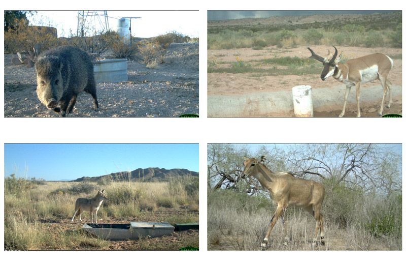
Some of the images provide excellent portraits of the animals. Figure 4 shows four examples.

Figure 4. Example trail camera images. Clockwise from bottom left: coyote, javelina, pronghorn, and nilgai.
Javelina are found in Central and South America and the southwestern portions of North America. They resemble wild boar but are a distinct species. Pronghorn and coyotes are common at most of our sites. Nilgai are ubiquitous in India, where Hindus regard them as sacred. They were introduced into Texas in the 1920s. The only place they are found in our sites is Laguna Atascosa NWR.
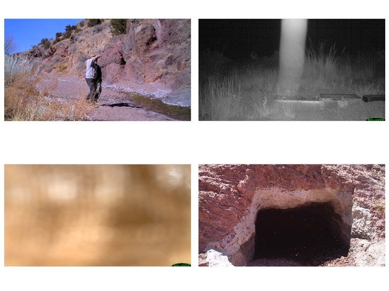
About one-third of the images were taken at night with infrared, and appear in grayscale, like the top two examples shown in Figure 5.

Figure 5. Top: two grayscale infrared images. Bottom: two full-color images of an oryx.
The two oryx images were easily classified by human experts, even though the images show very different views. Traditional image processing techniques, which would look for features like number of legs, presence and style of antlers, and type of tail, would be baffled by the badly lit closeup on the bottom right.
There are thousands of images triggered by nonwildlife activity, including humans, cows, horses, vehicles, and domestic animals. In Figure 6, the image on the upper right has been classified as a ghost.

Figure 6. Images triggered by nonwildlife activity. Top: A human (left) and a “ghost” (right). Bottom: “unidentified” images.
The subject in the lower left is obviously too close to the camera. There are faint yellow specks in the lower-right image that could be a swarm of small flying insects. Both images are classified as “unidentified.”
Training Our Deep Learning Network
Inception-v3 is a convolutional neural network (CNN) that is widely used for image processing. We will use a version of the network pretrained on more than a million images from the ImageNet database. Inception-v3 is an off-the-shelf image CNN. There is nothing in it specifically for trail cameras. We choose a random sample of 1400 from each of our 40 species and designate 70% (980) as training images and 30% (420) as validation images. We let the training run overnight on a Linux® machine with a GPU (Xeon® E5-1650v4 processor, 3.5 GHz, 6 HT cores, 64 GB RAM, and a 12 GB NVIDIA® Titan XP GPU).
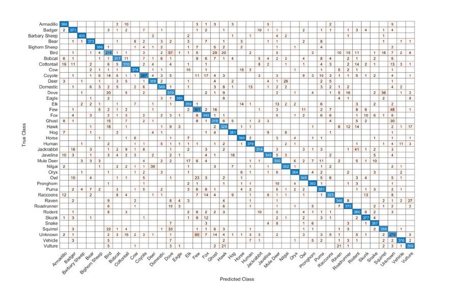
The resulting confusion chart (Figure 7) is a 40-by-40 matrix A where a(k,j) is the number of times an observation in the k-th true class was predicted to be in the j-th class. If the classification worked perfectly, the matrix would be diagonal. In this experiment, the values on the diagonal would all be 420. Nearness to diagonal is a measure of accuracy:
accuracy = sum(diag(A))/sum(A,'all') = 0.8686
Many of the large off-diagonal elements are not surprising. The smallest diagonal value, 216, is for birds. The row labeled Bird shows that the predicted class is often some other species. The next smallest diagonal element, 270, is for unknown. There is confusion between unknown and other species. Coyotes, with a diagonal value of 297, do not fare well, perhaps because they often appear in ambiguous images. Deer and nilgai, with diagonal values of 358 and 352, have good overall accuracy but are confused with each other.
On the other hand, the animals that are correctly classified the most often include the barbary sheep, whose diagonal value is 405. Eagles, horses, and pronghorn are correctly classified 390 or more times. The bighorn sheep has a 386.
Testing the CNN on Unclassified Images
We now have a CNN trained to classify trail camera images. How does it perform at a new location with images that have never been classified? We sample every tenth image from the Armendaris ranch, a total of 18,242. The CNN classification found 39 different species.
Almost half of the classifications—8708—were for bighorn sheep. Only 454 were for mule deer. This surprised me at first, because it meant that the network was predicting that Armendaris has almost 20 times as many bighorn sheep as mule deer, while Sevilleta, less than 100 miles to the north, has the opposite: 40 times as many mule deer as bighorn sheep.
But this result doesn’t surprise Jim Sanderson. The mountains on Armendaris are the natural habitat for the sheep. The ranch manages the bighorn sheep in the same way that it manages its buffalo herds. Hunting bighorn rams is an important source of income for the ranch.
The CNN classification labels 93 images as pumas. This appears to be an overestimate. Examination of the 93 images reveals only 10 or 11 of the elusive animals.
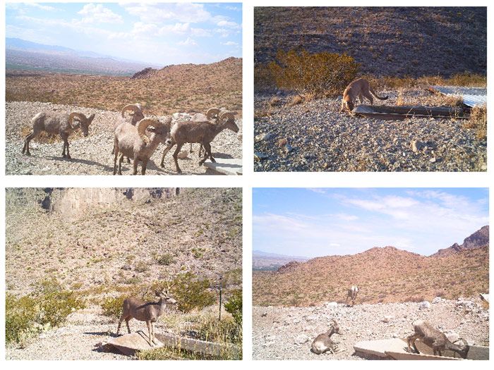
All four images in Figure 8 are from Armendaris. The upper two are correctly classified by the CNN as bighorn sheep and puma, respectively. But the lower two receive the same classifications; that is clearly incorrect.

Figure 8. Classification of previously unclassified images from the Armendaris ranch. The upper images are classified by the CNN as bighorn sheep and puma, evidently correctly. The lower images are also classified as bighorn sheep and puma, apparently incorrectly.
Conclusion
Overall, this deep learning classifier is more successful than I would have predicted. Even in its current state, it may be useful to investigators. Any further development of our CNN should focus on designing features specific to trail camera image identification.
One thing is clear—the more data the better. The 5 million images collected by the Fish and Wildlife Service were essential for training a network to this level of accuracy.
Acknowledgements
Thanks to Jim Sanderson, to Grant Harris at the Albuquerque FWS, and to Heather Gorr, Johanna Pingel, and the MathWorks News & Notes editorial team.
Published 2020


