Analytical Modeling of Aircraft Wing Loads Using MATLAB and Symbolic Math Toolbox

When modeling engineering systems, it can be difficult to identify the key parameters driving system behavior because they are often buried deep within the model. Analytical models can help because they describe systems using mathematical equations, showing exactly how different parameters affect system behavior.

In this article, we will derive analytical models of the loads and bending moments on the wing of a small passenger aircraft to determine whether the wing design meets strength requirements. We will derive the models in the notebook interface in Symbolic Math Toolbox™. We will then use the data management and analysis tools in MATLAB^® to simulate the models for different scenarios to verify that anticipated bending moments are within design limits.

While this example is specific to aircraft design, analytical models are useful in all engineering and scientific disciplines –for example, they can be used to model drug interactions in biological systems, or to model pumps, compressors, and other mechanical and electrical systems.

Analytical Modeling of Wing Loads

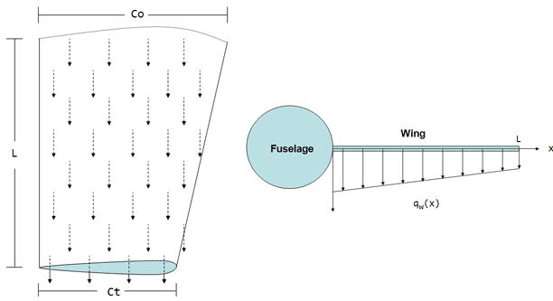
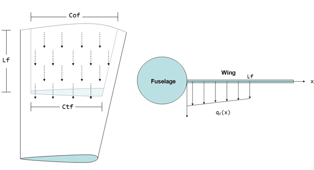
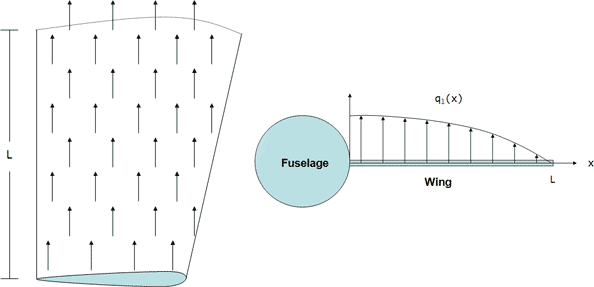
We will evaluate the three primary loads that act on the aircraft wing: aerodynamic lift, load due to wing structure weight, and load due to the weight of the fuel contained in the wing. These loads act perpendicular to the wing surface, and their magnitude varies along the length of the wing (Figures 1a, 1b, and 1c).

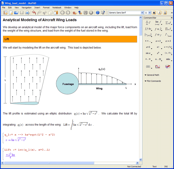
We derive our analytical model of wing loads in the Symbolic Math Toolbox notebook interface, which offers an environment for managing and documenting symbolic calculations. The notebook interface provides direct support for the MuPAD language, which is optimized for handling and operating on symbolic math expressions.

We derive equations for each load component separately and then add the individual components to obtain total load.

Lift

We assume an elliptical distribution for lift across the length of the wing, resulting in the following expression for lift profile:

\[q_1(x) = ka\sqrt{L^2 - x^2}\]

where

\(L\) = length of wing
\(x\) = position along wing
\(ka\) = lift profile coefficient

We can determine the total lift by integrating across the length of the wing

\[\text{Lift} = \int_0^L ka \sqrt{L^2 - x^2} \mathrm{d}x\]

Within the notebook interface we define \(q_1(x)\) and calculate its integral (Figure 2). We incorporate math equations, descriptive text, and images into our calculations to clearly document our work. Completed notebooks can be published in PDF or HTML format.

Through integration, we find that

\[\text{Lift} = \frac{\pi L^2 ka}{4}\]

We determine \(ka\) by equating the lift expression that we just calculated with the lift expressed in terms of the aircraft’s load factor. In aircraft design, load factor is the ratio of lift to total aircraft weight:

\[n = \frac{\text{Lift}}{W_{to}}\]

Load factor equals 1 during straight and level flight, and is greater than 1 when an aircraft is climbing or during other maneuvers where lift exceeds aircraft weight.

We equate our two lift expressions,

\[\frac{W_{to} n}{2} = \frac{\pi L^2 ka}{4}\]

and solve for the unknown \(ka\) term. Our analysis assumes that lift forces are concentrated on the two wings of the aircraft, which is why the left-hand side of the equation is divided by 2. We do not consider lift on the fuselage or other surfaces.

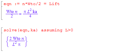
Plugging \(ka\) into our original \(q_1(x)\) expression, we obtain an expression for lift:

\[q_1(x) = \frac{2 W_{to} n \sqrt{L^2 - x^2}}{L^2 \pi}\]

An analytical model like this helps us understand how various parameters affect lift. For example, we see that lift is directly proportional to load factor (n) and that for a load factor of 1, the maximum lift

\[\frac{2 W_{to}}{\pi L}\]

occurs at the wing root (\(x=0\)).

Weight of Wing Structure

We assume that the load caused by the weight of the wing structure is proportional to chord length (the width of the wing), which is highest at the wing base (\(C_o\)) and tapers off toward the wing tip (\(C_t\)). Therefore, the load profile can be expressed as

\[q_w(x) = kw\left(\frac{C_t - C_o}{L} x + C_o\right)\]

We define \(q_w(x)\) and integrate it across the length of the wing to calculate the total load from the wing structure:

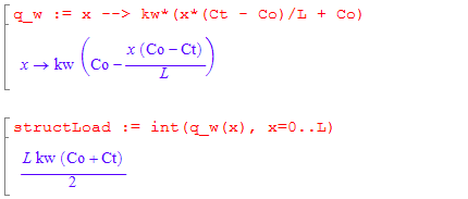
We then equate this structural load equation with the structural load expressed in terms of load factor and weight of the wing structure (\(W_{ws}\))

\[\frac{W_{ws} n}{2} = \frac{kw L (C_o + C_t)}{2}\]

and solve for \(kw\).

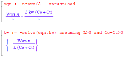
Plugging kw into our original \(q_w(x)\) expression, we obtain an analytical expression for load due to weight of the wing structure.

\[q_w(x) = - \frac{W_{ws} n \left(C_o - \frac{x(C_o - C_t)}{L}\right)}{L(C_o + C_t)}\]

Weight of Fuel Stored in Wing

We define the load from the weight of the fuel stored in the wing as a piecewise function where load is zero when \(x > L_f\). We assume that this load is proportional to the width of the fuel tank, which is at its maximum at the base of the wing (\(C_{of}\)) and tapers off as we approach the tip of the fuel storage tank (\(C_{tf}\)). We derive \(q_f(x)\) in the same way that we derived \(q_w(x)\), resulting in an equation of the same form:

\[q_f(x) = \begin{cases} 0 & \text{if } L_f < x\\ -\frac{W_f n \left(C_{of} - \frac{x(C_{of} - C_{tf})}{L_f}\right)}{L_f (C_{of} + C_{tf})} & \text{if } x \leq L_f\end{cases}\]

Total Load

We calculate total load by adding the three individual load components. This analytical model gives a clear view of how aircraft weight and geometry parameters affect total load.

\[q_t(x) = \begin{cases} \begin{split} &\frac{n}{L^2 \pi}\left(2 W_{to}\sqrt{L^2 - x^2}\right) \\ &\quad + \frac{n\left( -\pi C_o L W_{ws} + \pi C_o W_{ws} x - \pi C_t W_{ws} x\right)}{L^2 \pi (C_o + C_t)} \end{split} & \text{if } L_f < x\\ \begin{split} &\frac{2 W_{to} n \sqrt{L^2 - x^2}}{L^2 \pi} - \frac{W_{ws} n (C_t x - C_o x +C_o L)}{L^2 (C_o + C_t)} \\ &\quad - \frac{W_f n (C_{tf} x - C_{of} x + C_{of} L_f)}{L_f^2(C_{of} + C_{tf})} \end{split} & \text{if } x \leq L_f\end{cases}\]

Defining Model Parameters and Visualizing Wing Loads

We now have an analytical model for wing loads that we can use to evaluate aircrafts with various wing dimensions and weights. The small passenger aircraft that we are modeling has the following parameters:

\(W_{to}\) = 4800 kg (total aircraft weight)
\(W_{ws}\) = 630 kg (weight of wing structure)
\(W_f\) = 675 kg (weight of fuel stored in wing)
\(L\) = 7 m (length of wing)
\(L_f\) = 4.8 m (length of fuel tank within wing)
\(C_o\) = 1.8 m (chord length at wing root)
\(C_t\) = 1.4 m (chord length at wing tip)
\(C_{of}\) = 1.1 m (width of fuel tank at wing root)
\(C_{tf}\) = 0.85 m (width of fuel tank at Lf)

To evaluate load during the climb phase, we assume a load factor of 1.5, then plot the individual load components and total load (Figure 3).

We see that lift is the largest contributor to total load and that the maximum load of 545 N*m occurs at the end of the fuel tank. Fuel load also contributes significantly to the total load, while the weight of the wing is the smallest contributor.

While it is useful to visualize wing loads, what really concerns us are the shear force and bending moments resulting from these loads. We need to determine whether worst-case bending moments experienced by the wing are within design limits.

Deriving a Bending Moment Model

We can use the expression that we derived for load on the wing to calculate bending moment. We start by integrating total load to determine shear force:

\[V(x) = - \int q_t(x) \mathrm{d}x\]

Bending moment can then be calculated by integrating shear force:

\[M(x) = \int V(x) \mathrm{d}x\]

We write a custom function in the MuPAD language, CalcMoment.mu. This function accepts load profile and returns the bending moment along the length of the wing (Figure 4). Symbolic Math Toolbox includes an editor, debugger, and other programming utilities for authoring custom symbolic functions in the MuPAD language.

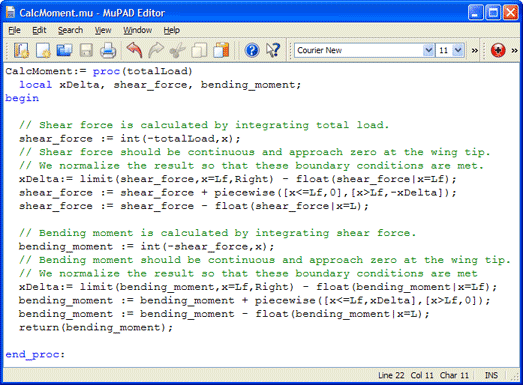
We use this function with the aircraft parameters that we defined previously to obtain an expression for bending moment as a function of length along wing (x) and load factor (n)

\[\begin{cases} \begin{split} &0.27 n x^3 - 2085.0 n x - 25.31 n x^2 - 1056.56 n \\  &\quad + 10695.21 n \left(0.14 x \arcsin(0.14x) + \sqrt{1.0 - 0.02 x^2}\right) \\ &\quad - 10.39 n \left(49.0 - 1.0 x^2\right)^{\frac{3}{2}}\end{split} & \text{if } 2.4 < x \\ \begin{split} &2.77 n x^3 - 1747.5 n x - 104.64 n x^2 - 1444.25 n \\  &\quad + 10695.21 n \left(0.14 x \arcsin(0.14x) + \sqrt{1.0 - 0.02 x^2}\right) \\ &\quad - 10.39 n \left(49.0 - 1.0 x^2\right)^{\frac{3}{2}}\end{split} & \text{if } x \leq 2.4 \end{cases}\]

As with wing loads, we plot bending moment assuming a load factor of 1.5 (Figure 5).

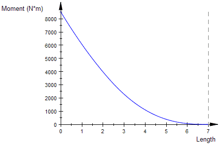
As expected, the bending moment is highest at the wing root with a value of 8.5 kN*m. The wing is designed to handle bending moments up to 40 kN*m at the wing root, but since regulations require a safety factor of 1.5, bending moments exceeding 26.7 kN*m are unacceptable. We will simulate bending moments for various operating conditions, including conditions where the load factor is greater than 1.5, to ensure that we are not in danger of exceeding the 26.7 kN*m limit.

Simulating Bending Moment in MATLAB

The bending moment equation is saved in our notebook as moment. Using the getVar command in Symbolic Math Toolbox, we import this variable into the MATLAB workspace as a sym object, which can be operated on using MATLAB symbolic functions included in Symbolic Math Toolbox.

bendingMoment = getVar(nb,’moment’);

Since we want to numerically evaluate bending moments for various conditions, we convert our sym object to its equivalent numeric function using the matlabFunction command.

h_MOMENT = matlabFunction(bendingMoment)

h_MOMENT is a MATLAB function that accepts load factor (n) and length along wing (x) as inputs. Because we’re evaluating bending moments at the wing root (x=0), load factor becomes the only variable that affects bending moments. As mentioned earlier, load factor is equal to Lift / Wto. Using the standard lift equation, and assuming the aircraft is not banking, load factor can be expressed as

\[n = \frac{\rho A C_L V^2}{2 W_{to}}\]

Where
\(\rho\) = air density —1.2 kg/m^3
\(A\) = planform area (approximately equal to total surface area of wings)—23 m^2
\(C_L\) = lift coefficient (varies with aircraft angle of attack, which ranges from 3 to 12 degrees)— 0.75 to 1.5
\(V\) = net aircraft velocity (accounts for aircraft speed and external wind conditions)—40 m/s to 88 m/s

We define these variables in MATLAB and evaluate h_MOMENT for the range of lift coefficients and aircraft velocities listed above. We store the results in a dataset array (Figure 6), available in Statistics and Machine Learning Toolbox™.

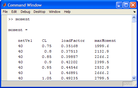
Dataset arrays provide a convenient way to manage data in MATLAB, enabling us to filter the data to view and analyze the subsets we are most interested in. Since we want to determine whether bending moments ever exceed the 26.7 kN*m threshold, we only need the bending moment data where the load factor is greater than 1.5. We filter the dataset and plot the data for these conditions (Figure 7).

moment_filt = moment(moment.loadFactor>1.5,:)
x = moment_filt.netVel;
y = moment_filt.CL;
z = moment_filt.maxMoment;
[X,Y] = meshgrid(x,y);
Z = griddata(x,y,z,X,Y);
surf(X,Y,Z)

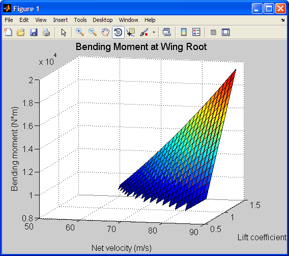
The plot shows that the peak bending moment, 19.3 kN*m, occurs when net aircraft velocity and lift coefficient are at their maximum values of 88 m/s and 1.5, respectively. This result confirms that bending moments will be safely below the 26.7 kN*m limit, even for worst-case conditions.

The Value of Analytical Modeling

Our analytical models gave us a clear view into how different aircraft parameters and operating conditions affect loads and bending moments on the aircraft wing. They enabled us to verify that the wing is able to withstand worst-case loading conditions that it could encounter during the climb phase of flight.

The models discussed in this article were used only for high-level proof-of-concept analysis, but analytical models could also be used for more detailed system modeling tasks—for example, to model the airflow near the leading edge or tip of the wing.