Atmospheric Carbon Dioxide Modeling and the Curve Fitting Toolbox

A common measurement for studying the effect of burning fossil fuels on weather patterns is the level of carbon dioxide (CO₂) concentration in the atmosphere. Some scientists believe the upward trend in CO₂ levels could cause atmospheric temperatures to rise, polar ice caps to melt, and climates of different regions of the earth to change radically.

Since this data has cyclical phenomena, as well as an upward growth trend, nonlinear fitting techniques are appropriate, but can require added effort when compared to fitting a linear model. However, with the right tools and knowledge of your data, you can quickly determine the coefficients of a nonlinear model.

This article describes how to fit a nonlinear model to available CO₂ data using the newly released Curve Fitting Toolbox.

Modeling the Data

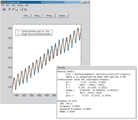
In this example, we use CO₂ data, in parts per million, collected by the U.S. National Oceanic and Atmospheric Administration (NOAA) from 1979 to 1996 at the Mauna Loa Observatory in Hawaii₂. The captured data is shown in the following illustration.

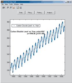
Cyclical phenomena in nature can be modeled by a sinusoid and its higher harmonics, that is,

A_kT/K and Φ_k are the amplitude, period, and phase, respectively, of the k-th harmonic. The sinusoidal terms capture seasonal trends, but the persistent upward trend requires an exponential term. A suggested model for this data, determined by examining records of total world fossil fuel production from the mid 1860s, is

where t (time) is in years, α is believed to be approximately 0.0444/year, and the other parameters are unknown (including the number of sinusoids needed)².

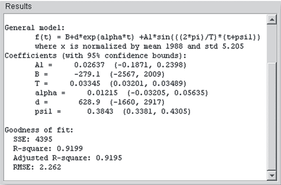
To build the model, we go to the Curve Fitting Toolbox's Fitting GUI and create a custom equation with one sinusoid term.

Because the time values are large, we can select the option to center and scale the time variable (remove the mean and divide by the standard deviation) to improve the conditioning of the numerical calculations.

Refining the Model

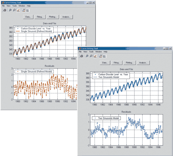
We can improve upon this model in several ways. First, we can determine the coefficients of the exponential term separately. We use the toolbox's built-in exponential model which automatically calculates optimal start points from the data,

Fitting this model results in coefficients of d = 349.6 and α = 0.02185. Using these values of d and a as start values in the sinusoidal model, we get a new fit that matches the cyclical nature well.

Now we can plot the residuals that still show a cyclical sinusoid pattern, so another sinusoid term is warranted.

Extending the Analysis

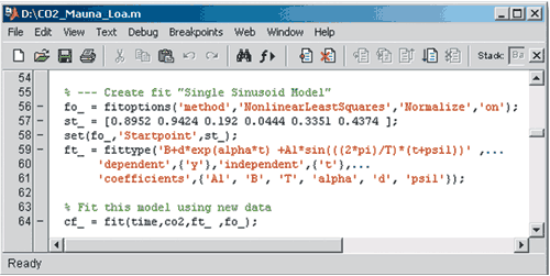
When we have found a satisfactory model, we can send our fits to the MATLAB workspace for further analysis. We have several other observatory sites to examine (e.g., Samoa, the South Pole, and Barrow) and so can generate an M-file function that can recreate our fits. Then we can call the function in a loop to automatically fit other data sets to see how the resulting models compare across observatory sites.

This example touches on a few of the features that will help you fit models to data. Whether the models are linear or nonlinear, the Curve Fitting Toolbox enables you to quickly fit standard models from its library or custom models you create.