Data-Driven Insights with MATLAB Analytics: An Energy Load Forecasting Case Study

Energy producers, grid operators, and traders must make decisions based on an estimate of future load on the electrical grid. As a result, accurate forecasts of energy load are both a necessity and a business advantage.

The vast amounts of data available today have made it possible to create highly accurate forecast models. The challenge lies in developing data analytics workflows that can turn this raw data into actionable insights. A typical workflow involves four steps, each of which brings its own challenges:

1. Importing data from disparate sources, such as web archives, databases, and spreadsheets
2. Cleaning the data by removing outliers, and noise, and combining data sets
3. Developing an accurate predictive model based on the aggregated data using machine learning techniques
4. Deploying the model as an application in a production environment

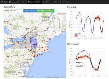
In this article, we will use MATLAB^® to complete the entire data analytics workflow for a load forecasting application. Using this application, utility analysts can select any region in the state of New York to see a plot of past energy load and predicted future load (Figure 1). They can use the results to understand the effect of weather on energy loads and determine how much power to generate or purchase. Given that the State of New York alone consumes several billions of dollars of electricity per year, the result can be significant for power generation companies.

Importing and Exploring Data

This case study uses two data sets: energy load data from the New York Independent System Operator (NYISO) website, and weather data—specifically, the temperature and dew point—from the National Climatic Data Center.

NYISO publishes monthly energy data in a ZIP file containing a separate comma-separated value (CSV) file for each day. The typical approach for working with data spread across several files is to download a sample file, explore it to identify the data values to be analyzed, and then import those values for the complete data set.

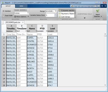
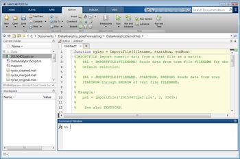
The Import Tool in MATLAB lets us select columns in a CSV file and import the selected data into a variety of MATLAB data structures, including vectors, matrices, cell arrays, and tables. The energy load CSV contains a time stamp, a region name, and a load for the region. With the Import Tool, we select CSV file columns and a target format. We can either import the data from the sample file directly or generate a MATLAB function that imports all files that match the format of the sample file (Figure 2). Later we can write a script that invokes this function to programmatically import all the data from our source.

Once the data has been imported, we generate preliminary plots to identify trends, reformat time and date stamps, and perform conversions—for example, by swapping the rows and columns in the data table.

Cleaning and Aggregating the Data

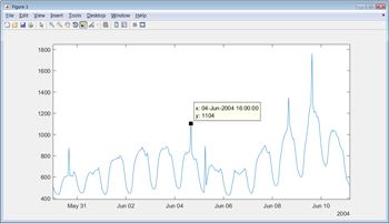
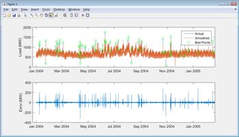
Most real-world data contains missing or erroneous values, and before the data can be explored, these must be identified and addressed. After reformatting and plotting the NYISO data, we notice spikes in load that fall outside the normal cyclical rise and fall of demand (Figure 3). We must decide whether these spikes are anomalous and can be ignored by the data model, or whether they indicate a phenomenon that the model should account for. We choose to examine only normal cyclical behavior for now; we can address the spikes later if we decide that our model needs to account for such behavior.

There are several ways to automate the identification of the spikes. For example, we can apply a smoothing spline and pinpoint the spikes by calculating the difference between the smoothed and original curves (Figure 4).

After removing the anomalous points from the data, we must decide what to do about the missing data points introduced by their removal. We could simply ignore them; this has the advantage of reducing the size of the data set. Alternatively, we could substitute approximations for the missing values in MATLAB by interpolating or using comparable data from another sample, taking care not to bias the data. For the purposes of estimating load, we will ignore the missing values. We will still have enough “good” data to create accurate models.

After cleaning the temperature and dew point data using similar techniques, we aggregate the two data sets. Both data sets are stored in MATLAB table data types. We apply a table join in MATLAB by invoking the outerjoin function. The result is a single table giving us easy access to the load, temperature, and dew point for each time stamp.

Building a Predictive Model

MATLAB provides many techniques for modeling data. If we know how different parameters influence the energy load, we might use statistics or curve fitting tools to model the data with linear or nonlinear regression. If there are many variables, the underlying system is particularly complex, or the governing equations are unknown, we could use machine learning techniques such as decision trees or neural networks.

Since load forecasting involves complex systems with many variables to be considered, we’ll opt for machine learning—specifically, supervised learning. In supervised learning, a model is developed based on historical input data (the temperature) and output data (the energy load). After the model is trained, it is used to predict future behavior. For energy load forecasting, we can use a neural network and Deep Learning Toolbox™ to complete these steps. The workflow is as follows:

For this example, we opted for just one model. For most real-word applications, you would try several different machine learning models and evaluate their performance on training and test data. Statistics and Machine Learning Toolbox™ provides a variety of machine learning approaches, all using a similar calling syntax, making it easy to try out different approaches. The toolbox also includes the Classification Learner app for interactively training supervised learning models.

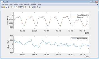
When the training is complete, we can use the test data to see how well the model performs on new data (Figure 5).

To automate the steps of setting up, training, and testing the neural network we use the Neural Fitting app to generate MATLAB code that we can invoke from a script.

To test the trained model, we run it against the data that we held in reserve and compare its predictions with the actual measured data. Results show that the neural network model has a mean absolute percent error (MAPE) of less than 2% on the test data.

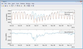
When we first run our model against a test data set, we notice a few instances where the model’s predictions diverge significantly from the actual load. Around holidays, for example, we see deviations from predicted behavior. We also notice that the model’s prediction for load on October 29, 2012, in New York City is off by thousands of megawatts (Figure 6). A quick Internet search shows that on this date Hurricane Sandy disrupted the grid across the region. It makes sense to adjust the model to handle holidays, which are regular and therefore predictable occurrences, but a storm like Sandy is a one-off event and therefore difficult to account for.

The process of developing, testing, and refining a predictive model often requires numerous iterations. Training and testing times can be reduced by using Parallel Computing Toolbox™ to run several steps simultaneously on multiple processor cores. For very large data sets you can scale up by running the steps on many computers with MATLAB Parallel Server™.

Deploying the Model as an Application

Once the model meets our accuracy requirements, the final step is moving it into a production system. We have several options. With MATLAB Compiler™ we can generate a standalone application or spreadsheet add-in. With MATLAB Compiler SDK™ we can generate .NET and Java^® components. With MATLAB Production Server™ we can deploy the application directly into a production environment capable of serving a large number of users simultaneously.

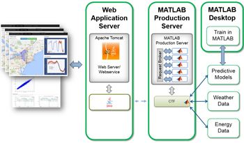
For our load prediction tool, we made the data analytics developed in MATLAB accessible via a RESTful API, which returns both numerical predictions and plots that can be included in an application or report. With the Production Server Compiler app we specify the MATLAB functions that we want to deploy. The app automatically performs a dependency analysis and packages the necessary files into a single deployable component. Using MATLAB Production Server we deploy the component as a processing engine, making the analytics available to any software or device on the network, including web applications, other servers, and mobile devices (Figure 7).

Next Steps

The energy load forecast model developed here provides highly accurate forecasts that can be used by decision-makers via a web front end. Because the model has been validated over months of test data, we have confidence in its ability to give a 24-hour forecast within 2% of actual load.

The model could be expanded to incorporate additional data sources, such as holiday calendars and severe weather alerts. Because the entire data analytics workflow is captured in MATLAB code, additional sources of data can easily be merged with the existing data, and the model retrained. Once the new model is deployed to MATLAB Production Server, the algorithm behind the load forecasting application is automatically updated—end users don’t even need to refresh the web page.