Nonlinear Mixed-Effects Modeling of Population Pharmacokinetics Data

Data sets involving nonlinear, sparse grouped data are common in the health sciences, especially in drug trials, where they are used to measure drug absorption, distribution, metabolism, and elimination. In this approach, patients are grouped using characteristics such as age, sex, weight, and smoking history. Given the expense of drug trials, however, it is not always possible to obtain sufficient patient data.

Nonlinear mixed-effects (NLME) modeling provides a good solution for modeling sparse datasets. These models account for both fixed effects (population parameters assumed to be constant each time data is collected) and random effects (sample-dependent random variables). In modeling, random effects act like additional error terms, and their distributions and covariances must be specified. Mixed-effects models provide a reasonable compromise between ignoring data groupings entirely, thereby losing valuable information, and fitting each group with a separate model, which requires significantly larger sample sizes.

Using population pharmacokinetics (popPK) data as an example, this article demonstrates a workflow for implementing a nonlinear mixed-effects model using SimBiology™.

The Phenobarbital Case Study¹

This well-known case study involved 59 pre-term infants who were given phenobarbital to prevent seizures during the first 16 days after birth. We will use the data collected during this study to estimate model parameters to best fit this data. This involves visualizing and preprocessing data, creating a PK model, fitting the model to data, and analyzing the results.

Visualizing and Preprocessing the Data

Data visualization and preprocessing reveals patterns in and distributions of the data. It also lets us deal with outliers and with bad or missing data points. For example, we may want to determine what type of elimination route phenobarbital has from this infant population, or look at the ranges of concentrations for each time point.

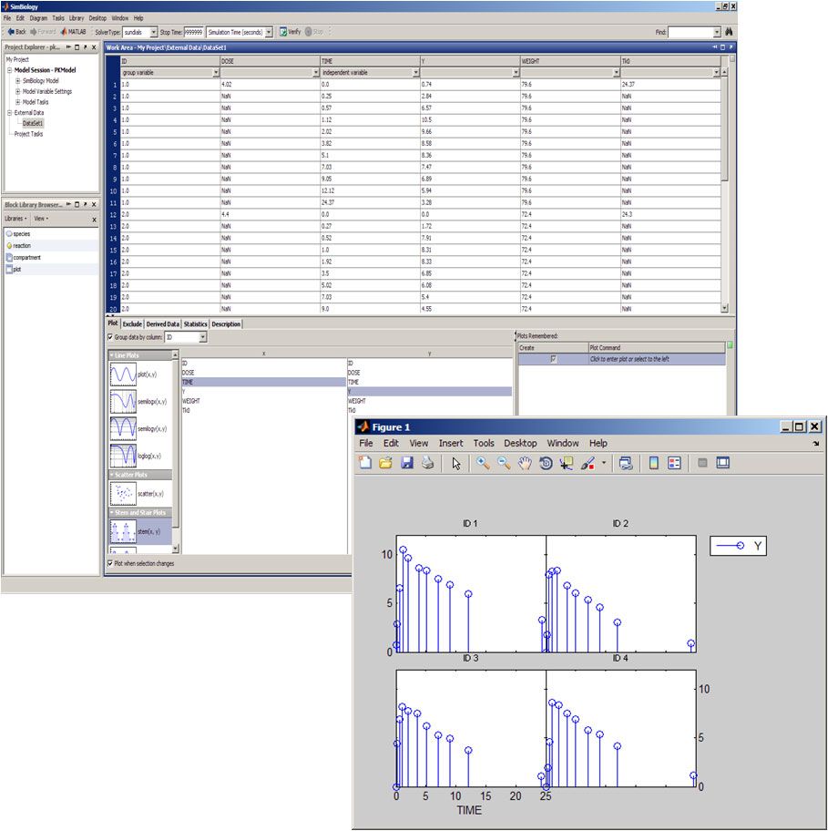
Data can be imported from a number of sources, including text files, Excel files, MAT files, and the MATLAB^® workspace. If a data file has common headers, such as ID or Time, SimBiology automatically recognizes and stores the headers as the group and independent variables.

To visualize the data, we select a plot type and an x and y variable in the external data panel in SimBiology (Figure 1). Plots are automatically updated as we select different variables or plots, and can be saved for later reuse. We can call MATLAB functions to create additional plots.

The exclude tab lets us remove outliers or bad data points either by selecting rows in the data table or by specifying rules. For example, to exclude all data pertaining to a specific patient, we can use a rule to remove all data points associated with that subject. Excluding a data point does not remove it from the dataset permanently, but rather flags the data point to be ignored during analysis. We can create new columns of data based on existing columns, and perform statistical analyses on the data, such as calculating the mean, area under the curve (AUC), area under the first moment curve (AUFMC), and mean residence time (MRT).

Creating a PK Model

We begin by defining the core of a PK model, the base model. This often consists of a number of compartments, a dosing type, and an elimination route. We may have a priori knowledge about the base model, or observe a trend in our data that will suggest where to start with a component. If we have no trends or prior knowledge, we can experiment with different base models and see what works best.

Because the data in our example appears to have a linear elimination route, we’ll use a simple one-compartment model with bolus intravenous dosing and linear clearance elimination.

We create the base model in SimBiology by entering the model components in the Model Wizard (Figure 2). Alternatively, we could create a blank model, import a model from a file, or import a model from the MATLAB workspace.

Fitting the Model to Data

In this step, we estimate model parameters based on the external data. In our example, we want to estimate the volume of the compartment (Central) and the parameter representing the clearance of the drug from the compartment (Cl-Central). We will need to calculate random effects for both.

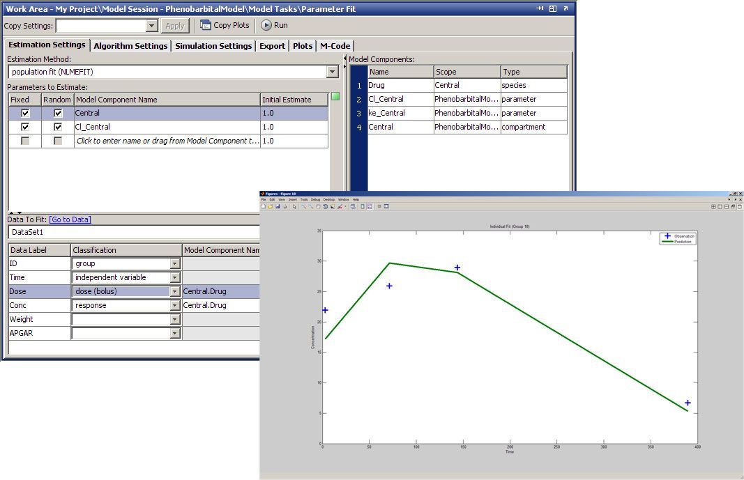
In the Fit Parameters task on the SimBiology desktop (Figure 3), we specify parameters that we want to estimate, parameters for which we want to calculate random effects, and the dataset to fit to. We also perform dataset mapping to identify group and independent variables and specify the covariance pattern. We click Run to begin the parameter fit.

Analyzing the Results

After fitting our model to the data, we’ll want to determine how well our fitting performed. SimBiology generates two types of outputs: a data panel summarizing the results, and diagnostic plots specified in the Fit Parameters task. The data panel includes log-transformed fixed estimates for the parameters, a list of the random effects for each parameter for each patient, a summary of statistics on the fit, and the estimated covariance matrix. We could make this an iterative workflow by examining the goodness-of-fit statistics, such as Akaike and Bayesian information criteria (AIC and BIC, respectively), from various models and selecting the one that best fits our data set.

The SimBiology desktop offers several prepackaged diagnostic plot types, including trellis plots, which plot both the observed and predicted time courses of drug concentration for each patient. The plot in Figure 3 shows that the predicted results accurately replicate the observed data for four of the subjects. Other plot types include observed versus predicted concentration values, box plots of the random effects calculated for each parameter, residual errors over time, and the distribution of residuals.

We can quickly capture our work by automatically creating an HTML or XML report in the SimBiology report generator. The report will be stored as a node in the SimBiology project. A SimBiology project stores multiple models, datasets, reports, analysis tasks, and all other components used in the workflow in one file, making it easy to manage and organize associated data files, models, and results.

Extending This Approach

We looked at a simple popPK example, but there are many possibilities for further modeling and analysis. For example, we could incorporate parallel computing to increase performance, leverage the SimBiology command line to include covariates in our model, and incorporate MATLAB code to customize or automate the workflow.

The author would like to thank Priya Moorthy, Sam Roberts, and Sowmini Sampath for their contribution to the example on which this article is based.

¹Grasela TH Jr, Donn SM. "Neonatal population pharmacokinetics of phenobarbital derived from routine clinical data." Dev Pharmacol Ther 1985:8(6). 374-83. PubMed Abstract