Simulating the Ramsey-Cass-Koopmans Model Using MATLAB and Simulink
By Sonia Bridge and Ken Deeley, MathWorks
Many economic and financial models, such as those for resource allocation or optimal growth, involve systems of differential equations with no explicit analytical solution. Solving these systems numerically and visualizing results are important tasks for economists and other financial analysts.
Using the fundamental Ramsey-Cass-Koopmans (RCK) model as an example, this article describes two workflows for creating, simulating, and visualizing a system of ordinary differential equations (ODEs). One approach is based on MATLAB®, the other on Simulink®. The MATLAB approach uses programming techniques familiar to financial professionals who work in a technical computing environment. The Simulink approach offers a visual modeling environment and graphical representation of the system.
Simulink is a block diagram environment used for modeling time-varying systems with feedback. Such systems are typical in control engineering applications, which for many years have influenced economic modeling [1]. Economic models can involve large-scale systems of ODEs with many equations and dependencies. Simulink provides convenient features such as subsystems and model referencing to support the modeling of large systems.
The code and models used in this article are available for download.
The Ramsey-Cass-Koopmans Model
The RCK model aims to explain long-term economic growth in terms of capital accumulation and consumption growth [2-4]. The core RCK model is two-dimensional, comprising two coupled ODEs for per-capita wealth (k) and per-capita consumption (c). Figure 1 shows the phase portrait of the system.
The core RCK model equations for per-capita wealth (k) and per-capita consumption (c) are:
\[\frac{dk}{dt} = f(k) - c - (\phi + \xi + \delta)k,\quad \frac{dc}{dt} = c \left(\frac{f'(k) - \theta - \xi - \delta}{\rho} - \phi \right)\]
Since k and c appear in both equations, the two ODEs are coupled. The terms in these equations are as follows:
- \(f(k) = k^{\alpha}\) is a production function measuring the relative economic output in terms of \(k\) and a capital elasticity parameter \(\alpha\) (the responsiveness of the output production to changes in the input capital).
- \(\phi\) is the growth rate of labor productivity (for example, due to technological innovation or efficiency improvements).
- \(\xi\) is the growth rate of labor supply (for example, due to migration or population increase).
- \(\delta\) is the depreciation rate of capital (for example, due to inflation).
- \(f'(k) = \alpha k ^{\alpha - 1}\) is the rate of change (derivative) of the production function \(f(k)\).
- \(\theta\) is an elasticity parameter indicating the tendency of consumers to smooth out their consumption over time.
- \(\rho\) is the rate at which consumers discount their future consumption (for example, by indicating a preference for immediate consumption or attempting to preserve their long-term average consumption).
Creating the RCK Model Using MATLAB
We can solve many systems of ODEs directly using the MATLAB function ode45, provided we express the system in the standard form \(\frac{dY}{dt} = G(t,Y)\) on the time interval \([t_0, t_f]\), and subject to the initial condition \(Y(0) = Y_0\). Note that \(Y\) and \(G(t,Y)\) are vector-valued if there are multiple unknown functions of time in the system of equations.
We begin by defining the model parameters in a structure variable params, and then write a vector-valued function RCK_Equations representing the right-hand side of the standard differential equation \(\frac{dY}{dt} = G(t,Y)\). This function returns a two-element vector containing the values of \(\frac{dk}{dt}\) and \(\frac{dc}{dt}\)at each time step.
We also write two auxiliary functions RCK_f and RCK_df returning the values of the production function \(f(k)\) and its derivative \(f'(k)\) respectively. We save each function in a separate file so that it will be easy to investigate the effect of different production functions on the numeric results.
function dY_dt = RCK_Equations(t, Y, params)
%RCK_EQUATIONS Function defining the right-hand sides of the two
%coupled ordinary differential equations defining the Ramsey-Cass-
%Koopmans model.

% Extract k and c.
k = Y(1);
c = Y(2);

% Write down the equations for dk/dt and dc/dt.
dY_dt(1, 1) = RCK_f(k, params) - c - ...
              (params.phi + params.xi + params.delta) * k; % dk/dt

dY_dt(2, 1) = ( ( RCK_df(k, params) - params.theta - params.xi - ...
             params.delta ) / params.rho - params.phi ) * c; % dc/dt

end % RCK_Equations
The next step is to create a function handle (@) containing the input function for ode45 by parameterizing RCK_Equations with the predefined parameters structure params. This function has to be a function of time (t) and state (Y) only.
RCK_Fun = @(t, Y) RCK_Equations(t, Y, params);
We ensure that both per-capita wealth and consumption remain nonnegative over time by modifying the solver options with odeset.
opts = odeset('NonNegative', [1, 2]);
Taking the initial conditions to be \(k_0 = 25\) and \(c_0 = 2\) and creating a time vector from 0 to 1.5 units, we can now solve the system numerically using ode45. The outputs of ode45 are time and state. Note that since we are creating a time vector t for ode45 directly, it is only necessary to return the second output argument Y from ode45.
Y0 = [25; 2];
t = linspace(0, 1.5, 5000);
[~, Y] = ode45(RCK_Fun, t, Y0, opts);
k_out = Y(:, 1); % Output per-capita wealth
c_out = Y(:, 2); % Output per-capita consumption
We use the MATLAB visualization function comet to create an animated trajectory of the solution path, showing the time evolution of capital and consumption. The final frame of this animation, superimposed on the phase plane, is shown in Figure 2. The red line is a small portion of the curve \(\frac{dk}{dt} = 0\) shown in Figure 1.
Finding the Steady States and Solving the System Using Time Elimination
We can find the steady state(s) of the system by solving the equations \(\frac{dk}{dt} = \frac{dc}{dt} = 0\). Solving \(\frac{dk}{dt} = 0\) yields the curve \(c^{*}(k)=f(k)-(\phi + \xi + \delta)k\) (the red curve in Figure 1). Solving \(\frac{dc}{dt} = 0\) yields a single value for \(k\), namely.
\[\hat{k} = \left(\frac{\alpha}{\rho\phi + \theta + \xi + \delta}\right)^{\frac{1}{1 - \alpha}}\]
This value defines the vertical line \(k = \hat{k}\) in Figure 1. We can use the meshgrid function to create lattices K and C of capital/consumption grid points. After computing the differentials dK and dC as defined by the RCK equations, we can then use the streamslice visualization function to render the streamlines in the \((k,c)\) plane.
streamslice(K, C, dK, dC)
Overlaying the curves \(c^{*}\) and \(k = \hat{k}\) creates the phase portrait shown in Figure 1.
As Carrol shows [3], there is no analytical solution for the model’s transition to its steady state. However, we can use the time elimination technique to obtain the following:
\[\frac{dc}{dk} = \frac{dc/dt}{dk/dt} = \frac{c(f'(k) - \theta - \xi -\delta - \phi\rho)}{\rho (f(k) - c - (\phi + \xi + \delta)k)}\]
Integrating with respect to k gives a solution trajectory for \(c\) as a function of \(k\). To avoid problems evaluating \(\frac{dc}{dk}\) when its numerator or denominator are zero, we split the \(k\)-domain into two parts, one to the left of \(\hat{k}\) and one to the right [2]. Applying ode45 gives the solution trajectory (Figure 3).
Note that the upper solution path is smooth, whereas the lower solution path suffers from numerical instabilities in the vicinity of \(\frac{dk}{dt} = 0\), a characteristic of certain stiff systems. In our example, instead of using ode45, we will use a solver designed to handle stiff systems, such as ode15s. To improve the reliability of the solution trajectory, we compute the Jacobian of the system and pass it to the solver via odeset. The resulting smooth path is shown in Figure 4. For larger or more complex systems, we could use Symbolic Math Toolbox™ to compute analytic Jacobians without manual calculation.
Creating the RCK Model Using Simulink
We solved the RCK system in MATLAB using techniques familiar to financial analysts. We’ll now take a less familiar but more visual approach: we’ll implement the system dynamically using libraries of predefined blocks in Simulink.
In Simulink, data is represented as signals and as parameters. Signals are the lines connecting blocks, and represent time―varying data, such as the derivative \(\frac{dk}{dt}\). Parameters are system values stored inside blocks―for example, the initial condition \(k_0\).
When modeling ODEs in Simulink, we begin with the Integrator block from the Continuous library. This block numerically integrates its input signal (the derivative). Since the system has first-order derivatives for k and c, we use two integrator blocks. The initial conditions \(k_0 = 5\) and \(c_0 = 3\) are assigned as parameters inside the blocks (Figure 5).

Figure 5. Integrator blocks for k and c. The red lines indicate signals not yet connected to other blocks.
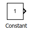
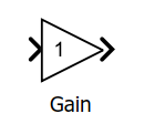
We implement the right-hand sides of the RCK equations using blocks from the Simulink library (Table 1).
| Block | Symbol | Purpose |
|---|---|---|
| Constant |

|
Reference model parameters (e.g., params.phi) |
| Product |

|
Multiply signals |
| Sum |

|
Add or subtract signals |
| Gain |

|
Multiply or divide a signal by a constant |
| Math Function |

|
Mathematical operations (e.g., powers and logarithms) |
| Outport |

|
Pass results to the MATLAB workspace (e.g., k and c) |
| Derivative |

|
Numerically approximate derivatives |
| Subsystem |

|
Group functionally related blocks |
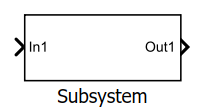
Table 1. Simulink blocks used to implement the right-hand sides of the RCK equations.
As our model increases in size and complexity, we can simplify it by grouping blocks into subsystems using the Subsystem block. We encapsulate the production function \(f(k)\) in a subsystem (Figure 6).

Figure 6. The production function \(f(k) = k^{\alpha}\) implemented as a subsystem.
We approximate the derivative \(f'(k)\) using the Derivative block. Note that the Derivative block has no initial condition parameter and so should not be used as a starting point for modeling ODEs.
Figure 7 shows the complete RCK model.
After constructing the model, we specify the simulation stop time as 500 time units and start the simulation. Figure 8 shows the resulting trajectory starting from the point \((k_0,c_0) = (5,3)\).
Running Simulations in Parallel
As part of the model analysis, we may want to investigate the dependency of the model on its parameters by running simulations using different sets of parameter values. Each simulation can be run independently and implemented in parallel using the parfor construct from Parallel Computing Toolbox™.
Starting with the MATLAB based model implementation, we create lattices of grid points K0 and C0 representing the different initial conditions we want to investigate. Within each iteration of the parfor loop, we select a different initial condition Y0 and store the outputs k_out and c_out using cell arrays.
RCK_Fun = @(t, Y) RCK_Equations(t, Y, params);
opts = odeset('NonNegative', [1, 2]);
t = linspace(0, 1.5, 1000);
parfor k = 1:numel(K0)
    % Initial values for per-capita wealth and consumption.
    Y0 = [K0(k); C0(k)];
    % Solve the coupled system.
    [~, Y] = ode45(RCK_Fun, t, Y0, opts);
    k_out{k} = Y(:, 1); % Output per-capita wealth
    c_out{k} = Y(:, 2); % Output per-capita consumption
end % parfor
Using 100-by-100 lattices of initial conditions means that we perform 10,000 parallel simulations of the model. These simulations produce the solution trajectories shown in Figure 9.
To simulate the Simulink RCK model in parallel we do the following:
- Load the model on each worker using
load_systemand thespmdconstruct. - Define arrays
K0andC0for the initial conditions under which we want to simulate the model. - Write a function to simulate the model programmatically using the
simcommand. (Note that to set parameters programmatically in the model usingset_param, we need to convert numerical values to text. Thetry/catchconstruct safeguards against unexpected convergence issues for isolated sets of initial conditions.) - Within each iteration of the
parforloop, call the function with a different pair of initial conditions.
%% Load the model once per worker.
spmd
    load_system('RCK_Model');
end % spmd

%% Perform the simulations in parallel.
parfor k = 1:numel(K0)

    simout(k) = runSim(K0(k), C0(k));

end % parfor

function simout = runSim(k0, c0)
% RUNSIM Function simulating the model for different initial values
% for per-capita wealth and consumption using the stiff system solver
% ode15s and a stop time of 45 time units.

% Format the initial values for per-capita wealth and consumption as text.
k0 = num2str(k0);
c0 = num2str(c0);
set_param('RCK_Model/capital', 'InitialCondition', k0)
set_param('RCK_Model/consumption', 'InitialCondition', c0)

% Run the simulation.
try
    simout = sim('RCK_Model', 'Solver', 'ode15s', 'StopTime', '45');
catch
    % If a simulation run fails to converge, assign an empty output.
    simout = Simulink.SimulationOutput;
end % try

end % runSim
Figure 10 shows the solution trajectories for 10,000 parallel simulations of the model.
Summary
In this article we demonstrated that a system of coupled ODEs can be simulated using either MATLAB or Simulink, and that each approach brings benefits.
Using MATLAB, we transformed the equations to the form required by ode45 and used function handles. Using the Integrator block in Simulink, we implemented the differential equations in their native form.
Both MATLAB and Simulink enable us to compute derivatives automatically. In MATLAB, we use the gradient function in Symbolic Math Toolbox. In Simulink, we use the Derivative block and the solver Jacobian configuration setting of ode15s.
Simulink simplifies the modeling of a large or complex system of ODEs. Subsystems help us to organize our model by grouping functionally related blocks The Simulink model window provides an intuitive visual layout of the model.
Both approaches enable parallelization. In both MATLAB and Simulink, we use the parfor construct. In Simulink, we use the sim command to simulate the model programmatically.
Both MATLAB and Simulink provide an integrated modeling environment for solving and visualizing systems of ODEs. The method you use depends on the size and complexity of your system of ODEs. Laying out the model using Simulink is quick, visual, and intuitive. If you are new to Simulink, plenty of resources are available on mathworks.com to help you get started.
Published 2016 - 93062v00
References
-
Christopher D. Carroll, “The Ramsey/Cass-Koopmans (RCK) Model,” November 2011


