The Watershed Transform: Strategies for Image Segmentation

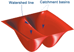
The term watershed refers to a ridge that divides areas drained by different river systems. A catchment basin is the geographical area draining into a river or reservoir.

So how are watersheds and catchment basins related to analyzing biological tissue, studying galaxies, or researching new semiconductor technology? And what is the connection to image processing?

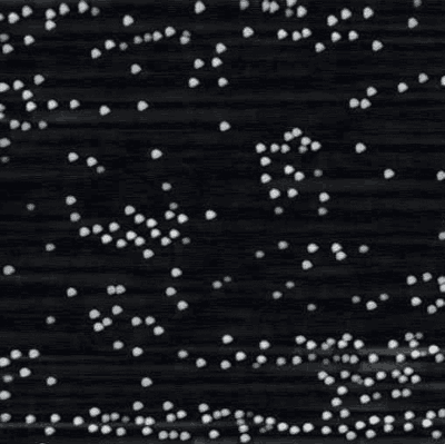
The connection is through computer analysis of objects in digital images. The objects could be anything: blood cells, stars, toner spots on a printed page, DNA microarray elements, or even quantum semiconductor dots, as in this image.

Computer analysis of image objects starts with finding them-deciding which pixels belong to each object. This is called image segmentation, the process of separating objects from the background, as well as from each other. R. Gonzalez and R. Woods write in their widely used textbook (Digital Image Processing) that "segmentation of nontrivial images is one of the most difficult tasks in image processing. Segmentation accuracy determines the success or failure of computerized analysis procedures."

The latest release (Version 3) of the Image Processing Toolbox includes new functions for computing and applying the watershed transform, a powerful tool for solving image segmentation problems.

Understanding the watershed transform requires that you think of an image as a surface. For example, consider the image below:

Example 1: Segmenting a Binary Image

Consider the task of separating the two touching objects in this binary image. How can we modify this image so its catchment basins are two circular objects?

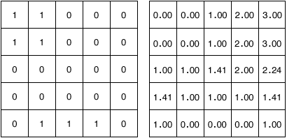
To do this we'll use another new tool in the Image Processing Toolbox: bwdist, which computes the distance transform. The distance transform of a binary image is the distance from every pixel to the nearest nonzero-valued pixel, as this example shows.

The distance transform of the binary image, computed using bwdist(BW), looks like image A (left).

This image is not very useful, because there is only one catchment basin spanning the entire image. Instead, try computing the distance transform of the image's complement:

D = bwdist(~BW); % image B (above)

This image is closer, but we need to negate the distance transform to turn the two bright areas into catchment basins.

D = -bwdist(~BW); % image C (above)

Now there is one catchment basin for each object, so we call the watershed function. L =

watershed(D);

L is called a label matrix, and it contains positive integers corresponding to the locations of each catchment basin. We can use the zero-valued elements of L, which are located along the watershed lines, to separate the objects in the original image.

BW(L == 0) = 0;
imshow(BW) % Segmented image D (above)

Example 2: Segmenting the Quantum Dots

The quantum dots image requires more work to make it suitable for watershed segmentation. First, we convert the image to grayscale and use a morphological top-hat operator (one of many new grayscale morphological tools) with a disk-shaped structuring element to smooth out the uneven illumination.

I = rgb2gray(RGB);
I2 = imtophat(I, strel('disk', 10));

Second, we use a new function called graythresh to determine a good threshold for converting the image to binary.

level = graythresh(I2);
BW = im2bw(I2,level);

Finally, we compute the distance transform of the complemented binary image, modify it to force the background to be its own catchment basin, and compute the watershed transform. The new function label2rgb is used to display the segmented objects using different colors.

D = -bwdist(~BW);
D(~BW) = -Inf;
L = watershed(D);
imshow(label2rgb(L,'jet','w'))

Example 3: Segmenting Steel Grains

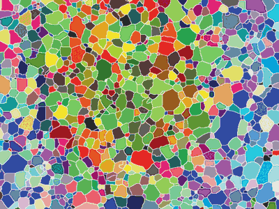
Our final example, a microscope image of steel grains, looks like a natural for watershed segmentation, since the light areas are already fairly well separated by dark lines.

We could simply compute the watershed of the complemented image.

L = watershed(imcomplement(I));

Unfortunately that doesn't work so well, as you can see below:

The result, oversegmentation, is a well-known phenomenon in watershed segmentation. Oversegmentation occurs because every regional minimum, even if tiny and insignificant, forms its own catchment basin. One solution is to modify the image to remove minima that are too shallow. That is exactly what the h-minima transform (imhmin) does.

I2 = imcomplement(I);
I3 = imhmin(I2,20); %20 is the height threshold for suppressing shallow minima
L = watershed(I3);

Here is the much improved result.

You have read about several ways to segment an image using the watershed transform. Another technique, known as marker-controlled watershed segmentation, is described on the Image Processing Toolbox page. To learn more about how to use the watershed transform in your own work, check out For Further Reading.

What's New in Image Processing Toolbox 3

The 63 new toolbox functions substantially extend its capabilities in these major areas:

• Grayscale morphology
• Spatial transformations
• Image registration
• Image deblurring
• DICOM import
• Multidimensional image processing
• Integer image arithmetic and filtering
• Tools that facilitate instrument control in an easy-to-use graphical environment
• Functions for determining your computer's available hardware
• Communication with multiple instruments within one MATLAB session

For more information about the new release, see the Image Processing Toolbox page.