Using Deep Learning for Predictive Maintenance of Underground Power Cable Systems

Underground power cable systems are less susceptible than overhead lines to windstorms, lightning, wildfires, ice storms, and other adverse weather events. They are more expensive to repair, however, and failures are more difficult to pinpoint and to restore. Left undetected, cable defects can cause power outages and danger to the public.

According to IEEE, approximately 90% of failures in underground cable systems are associated with partial discharge (PD), a phenomenon that occurs when the electric field within the cable exceeds the ability of the dielectric insulation to withstand it. When activated, PD produces high-frequency signals—typically, less than 100 millivolts in amplitude. Because these signals are symptomatic of dielectric deterioration and eventually fault, detecting them early can head off unexpected cable failures and allow for repair before the failure occurs. 

At IMCORP, we use MATLAB^® to design and train deep learning networks that accelerate and automate the process of detecting and characterizing PD signals. These networks not only detect PD signals; they also identify the approximate location of PD in the cable, the type of defect that produced it, and its severity (Figure 1).

Previous PD Analysis Approaches

We follow industry-standard quality control for manufacturers’ PD testing in which a higher-than-normal voltage is applied to an underground cable and to a coupler with an analog-to-digital converter (ADC) that captures high-frequency time-series signals. In the past, analysts processed the captured signals manually, looking for patterns that indicate the presence of PD. This process was both tedious and slow, and it sometimes produced inconsistent results and false positives. To make the analysts’ job easier, we implemented denoising and other digital signal processing algorithms, but the process remained highly subjective—even highly trained analysts with years of experience could sometimes reach different conclusions about the same signal.

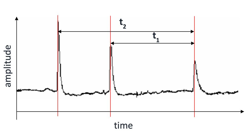
More recently, we began using machine learning to automate the classification of captured signals. We extracted features from the signal data in MATLAB, using signal processing algorithms to calculate the time between signal peaks and other features commonly used in PD analysis (Figure 2). We then used the Classification Learner App to train and evaluate classification models using a variety of methods, including logistic regression, support vector machine classification, random forest classification, and ensemble learning. The random forest model classified PD signals with 90% accuracy. The other models performed slightly better, giving about 92% accuracy. While these results were promising, we decided to explore deep learning to see whether it would increase classification accuracy.

Classifying PD Signals with Deep Learning

We applied two different approaches to classifying PD signals with deep learning networks. In the first, we trained a neural network using many of the extracted features we had used with our machine learning models. The network was trained on a data set of more than four million labeled instances of two dozen features. In the second approach, we trained a long short-term memory (LSTM) network directly on almost a million time-series signals previously analyzed and labeled by our team (Figure 3). Because our experience with deep learning was limited, we worked with MathWorks consultants, who helped us apply our domain expertise to design and train the neural network and the LSTM using the Deep Network Designer App.

After hyperparameter optimization, both networks classified PD signals with an accuracy of about 95%, a meaningful improvement over the machine learning models. To further improve accuracy, we augmented the time-series data by applying wavelet transforms and fast Fourier transforms. We saw a small improvement in accuracy (about 0.1%). Further model design and optimization in MATLAB is currently in progress.

Deep Learning for PD Location and Type Identification

For the second phase of the project, identifying the location of a PD source from an insulation defect within a cable, we trained two LSTM networks. One was trained to classify the source of the PD into any of 10 possible location ranges (equal-length cable segments), the other into 20 different location ranges. The maximum accuracy for both models was greater than 94% . We trained these two networks because we wanted to see whether the model accuracy remains constant with increased segmentation. After about 20 segments, accuracy started dropping.

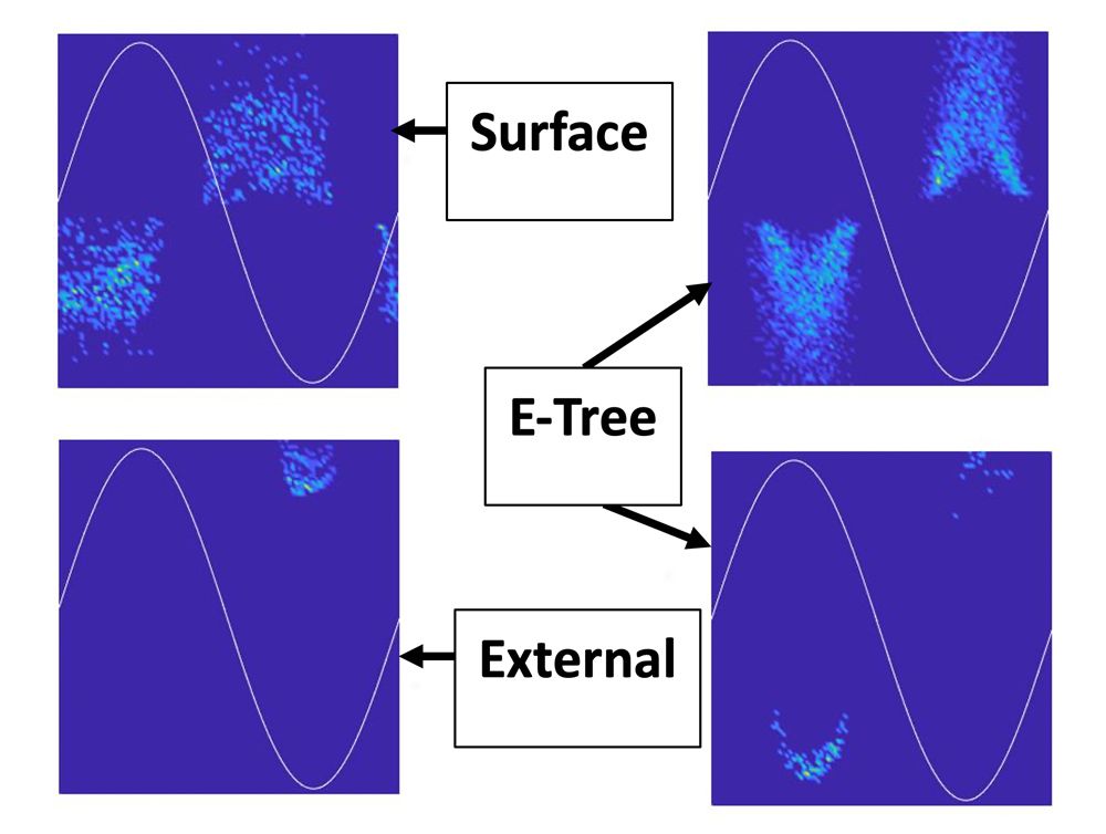
Finally, we trained a deep learning network to determine the type of defect producing the PD. Among the most common reasons for PD are workmanship, handling, and manufacturing. Typical types of PD defects include “termination PD,” “electrical treeing,” “void,” “interfacial PD,” and “external PD” (Figure 4). Of these, the electrical tree defect poses the highest risk of cable system failure. 

To classify a defect type, we analyzed the PD signals coming from a single defect and generated coded phase-resolved partial discharge (PRPD) plots. The pattens in PRPD plots vary depending on the type of defect: The PRPD plot for an electrical tree defect looks unlike the plot for a void defect, for example. 

For this part of the project, we used ResNet-50, a 50-layer convolutional neural network (CNN) pretrained on more than a million images. We retrained the CNN on a data set of more than 3,390 PRPD plots. It was then able to classify cable defect types with greater than 96% accuracy.

Planned Enhancements

Our deep learning networks provide results that rival the accuracy of highly trained signal analysts. They also provide a more consistent level of quality, as well as time savings for analysis and interpretation of up to 500% on complex data sets. As a result, our analysts are spending less time on monotonous signal analysis tasks and can focus on additional, equally important tasks.

Ultimately, we want our deep learning networks to perform classifications in near real-time so that technicians in the field can see the results soon after data is captured and rerun tests if needed. We are also working on expanding our training data set. IMCORP has one of the largest databases of PD signals in the world, with more than 120 million waveforms captured over many years of testing. We plan to use this data and the MATLAB interface for Databricks to enable large-scale training of deep learning models in the cloud.