Systems of Equations | Solving ODEs in MATLAB

Many mathematical models involve high order derivatives. But the MATLAB ODE solvers only work with systems of first order ordinary differential equations. So we have to rewrite the models to just involve first order derivatives. Let's see how to do that with a very simple model, the harmonic oscillator.

x double prime plus x equals 0. This involves a second order derivative. So to write it as a first order system, we introduced the vector y. This is a vector with two components, x, and the derivative of x.

We're just changing notation to let y have two components, x and x prime. Then the derivative of y is the vector with x and x double prime. So the differential equation now becomes y2 prime plus y1 equals zero. Do you see how we've just rewritten this differential equation. so y2 prime is playing of x double prime?

Once you've done that, everything else is easy. The vector system is now y1, y2 prime is y2 minus y1. The first components says y1 prime is y2. That's just saying that the derivative of the first component is the second. Here's the differential equation itself. Y2 prime is minus y1 is the actual harmonic oscillator differential equation.

When we write this as an autonomous function for MATLAB, here's the autonomous function. f is an autonomous function of t and y, that doesn't depend upon t. First it's a vector now, a column vector. The first component of f is y2. And the second component is -y1.

The first component here is just a matter of notation. All the content is in the second component, which expresses the differential equation.

Now for some initial conditions-- suppose the initial conditions are that x of 0 is 0, and x prime of 0 is 1. In terms of the vector y, that's y1 of 0, the first component of y is 0. And the second component is 1.

Or in vector terms, the initial vector is 0, 1. That implies they solution is sine t and cosine t. When we write the initial condition in the MATLAB, it's the column vector 0, 1.

Let's bring up the MATLAB command window. Here's the differential equation. y1 prime is y2. And y2 prime is -y1. Here's the harmonic oscillator.

We're going to integrate from 0 to 2pi, because they're trig functions. And I'm going to ask for output in steps of 2 pi over 36, which corresponds to every 10 degrees like the runways at an airport.

I'm going to need an initial condition. y0 not is 0. I need a column vector, 0, 1, for the two components. I'm going to use ODE45, and if I call it with no output arguments, ODE45 of the differential equation f, t span the time interval, and y0 the initial condition.

If I call ODE45 with no output arguments, it just plots the solution automatically. And here we get a graph of cosine t starting at 1, and sine t starting at 0.

Now if I go back to the command window, and ask to capture the output in t and y, I then get vectors of output. 37 steps, vector t, and two components y, the two columns containing sine and cosine. Now I can plot them in the phase plane.

Plot ya against y2. If I regularize the axes, I get a nice plot of a circle with small circles every 10 degrees, as I said, like the runways at an airport.

The Van der Pol oscillator was introduced in 1927 by Dutch electrical engineer, to model oscillations in a circuit involving vacuum tubes. It has a nonlinear damping term. It's since been used to model phenomena in all kinds of fields, including geology and neurology.

It exhibits chaotic behavior. We're interested in it for numerical analysis because, as the parameter mu increases, the problem becomes increasingly stiff. To write it as a first order system for use with the MATLAB ODE solvers, we introduce the vector y, containing x and x prime.

So y prime is x prime and x double prime. And then the differential equation is written so that the first component of y prime is y2. And then the differential equation is written in the second component of y.

Here's the nonlinear damping term minus y1. When mu is 0, this becomes the harmonic oscillator. And here it is as the anonymous function.

Let's run some experiments with the Van der Pol oscillator. First of all, I have to define the value of mu. And I'll pick a modest value of mu. Mu equals 100. And now with mu set, I can define the anonymous function.

It involves a value of mu. And here is the Van der Pol equation in the second component of f. I'm going to gather statistics about how hard the ODE solver works. And for that, I'm going to use ODE set, and tell it I want to turn on stats.

I need an initial condition. Now I'm going to run ODE45 on this problem. And I'm specifying just a starting value of t, and a final value of t. ODE45 is going to pick its own time steps. And I know with t final equals 460, it's going to integrate over it about two periods of the solution.

Now we can watch it go for a while. It's taking lots of steps. And it's beginning to slow down as it takes more and more steps. Now this begins to get painfully slow as it runs into stiffness.

I'll turn off the camera for a while here, so you don't have to watch all these steps. We're trying to get up here to 460. And I'll turn it back on as we get close to the end.

OK, well, the camera's been off about three minutes. And you can see how far we've gotten. We're nowhere near the end. So I'm going to press the stop button here. And we'll go back to the command window.

And oh, so we didn't get to the end here. Let me back off on the time interval and try this value here. See how that works. So this is going to still take lots of steps.

But we'll be able to-- This will go over about one period. We'll actually get to the end here.

I'll leave the camera on until we finish. OK so that took a little under a minute. And it took nearly 15,000 steps. So let's run it with a stiff solver.

There. So it took half a second, and only 500 steps. So there's a modest example of stiffness here. So let's examine the Van der Pol equation using the stiff solver. Let's capture the output and plot it.

Because that plot wasn't very interesting. I want to plot it a couple of different ways. And again, I want to go back up to the-- capture a couple periods.

Let's plot one of the current components as a function of time. And here it is. Here's the Van der Pol equation.

And you can see it has an initial transient, and then it settles into this periodic oscillation with these really steep spikes here. And even this stiff solver is working hard at these rapid changes. We've got a fair number of points in here, as it is it chooses the step size.

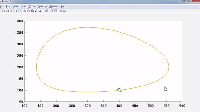
And now, let's go back to the command line and do a phase plane plot. So here's the phase plane plot of this oscillator with damping. And it's nowhere near a circle, which it would be if mu was 0.

And this is the characteristic behavior of the Van der Pol oscillator.