Frequency response design using sensitivity functions

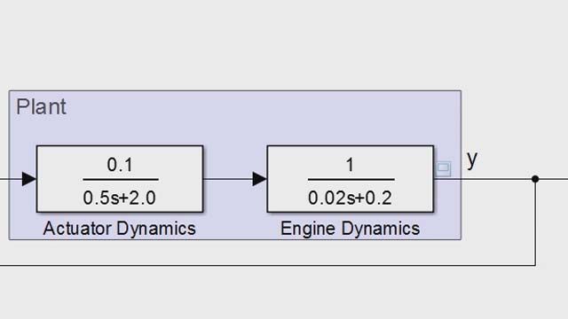
So now that we have a better feel for how the basic transfer function constructs look like in a frequency response diagram, and we understand how we can use superposition to combine them, I believe we are finally ready to start talking about how we can actually use any of this for designing controllers. In its most basic form, a control system will contain two main parts-- a plant, which represents the dynamics of the thing we're trying to control, and a controller. The plant dynamics can be modeled using fundamental principles or experimental data, or some combination of both.

The challenge from a control engineer's perspective is to, given those plant dynamics, come up with the appropriate thing to put in C such that the overall system-- plant and controller together-- behaves in some desired way. What we're looking at here is a system in an open-loop configuration. In the Laplace domain, all the components of a block diagram can be treated as algebraic terms, and complicated convolutional operations with signals become simple multiplications.

So, for this case, the output signal, y, is equal to the input signal, r, multiplied by C, and that result then multiplied by P. If what we want is our output, y, to track the desired reference, r, then we might think that the easiest solution will be to just make C the inverse of P. This will make y exactly equal to r, which, in principle, sounds like what we want, but in practice, is not a very good idea-- first of all, because most of the time, plant dynamics are not invertible. If the denominator has a higher order than the numerator, which is normally the case, trying to invert that will violate causality and cannot be implemented in a controller.

Also, it is very likely that your plant model will not be perfect. So even if you could cancel it out, your controller would not be accounting for any unmodeled dynamics. In addition, your plant may have unstable poles or zeros located on the right-hand side of the complex plane, and trying to directly cancel any of those can be a really bad idea. Finally, regardless of the controller we might choose, an open-loop configuration gives us no information on the output, y. So any unknown disturbance or noise that enters our system will show up unaffected on the output without the controller being able to do anything about them.

Adequately dealing with all these issues is one of the primary reasons why, most of the time, we need to use some form of feedback. Notice that by closing the loop, we are now making our controller respond to the difference-- or the error-- between the reference input signal and the system output signal. For this closed-loop architecture, y is equal to P times C times e, which can be substituted by (r-y). And just by doing a little algebra, we find that the closed-loop transfer function from the reference input, r, to the output, y, now becomes PC/(1+PC).

Similarly, if we look at the error, we find that the closed-loop transfer function from the reference input, r, to the error, e, is 1/(1+PC). These two transfer functions define the main characteristics of this closed-loop architecture. Even if we add a disturbance to our plant model, or some measurement noise to the system, and redo the algebra, we will find that the input signals-- in this case, r, d, and n-- end up propagating through the same two closed-loop transfer functions. PC/(1+PC) is called the complimentary sensitivity-- or, sometimes, that transmissibility transfer function, hence the T.

And, as you can see from the top equation, it directly affects how the reference signal, r, under the noise, n, will show up in the output signal, y. 1/(1+PC) is called the sensitivity transfer function-- or S. And, again, from the top equation, you can see that it directly affects how the disturbance, d, will show up in the output, y. It also shows how sensitive the error signal, e, is to all three input signals-- r, d, and n. In general, the frequency shape that we're going to be looking for in T should be something that resembles a low-pass filter like this.

Ideally, at low frequencies, we want a nice, flat gain of 0 dBs, as well as a phase shift that is as close to zero as possible. A flat 0 dBs gain on the low frequency means that our output signal, y, would very closely follow or track our desired signal reference, r, as long as the reference signal stays well below the system bandwidth. As a rule of thumb, the target system bandwidth should be 5 to 10 times the highest frequency we wish to track or control. The fast roll-off rate means that at any high-frequency noise, which should be well above the bandwidth, will be severely attenuated and will not affect our output signal, y.

The sharp drop in high frequencies in this closed-loop transfer function means that our system will have good high-frequency noise rejection characteristics. On the other hand, the corresponding frequency shape we will get for the sensitivity transfer function, S, will resemble a high pass filter like this. Good attenuation in the low-frequency range, well below the system bandwidth, means that any disturbances in that frequency range will not significantly affect our output signal, y. In other words, our system will have good frequency disturbance rejection characteristics.

It is worth noticing that these two transfer functions are not independent from each other, so they cannot be shaped arbitrarily. S and T will always add to 1—(PC+1)/(1+PC), regardless of C. So, as control engineers, we always need to be aware of the trade-offs between these two.