Evaluate Performance of NR Cell with Carrier Aggregation

Introduction to Carrier Aggregation

Carrier aggregation enables higher data rates by using multiple component carriers for simultaneous transmission and reception. This figure shows the carrier aggregation:

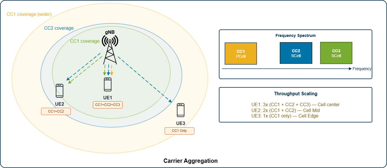
3GPP TS 38.300 describes three types of carrier aggregation:

When you configure carrier aggregation, one carrier acts as the Primary Cell (PCell) and the remaining carriers act as Secondary Cells (SCells). The PCell is established when you initially connect a UE to the gNB. You can then activate SCells for the carrier aggregation-capable UE nodes based on the traffic demand. A UE that does not support carrier aggregation connects only to the PCell and operates in single-carrier mode. For more information about carrier aggregation, see Carrier Aggregation in 5G System-Level Simulation.

Carrier aggregation also requires the NR nodes to distribute transmit power across component carriers. You can accomplish this by distributing the total node transmit power across the component carriers in proportion to their channel bandwidths. For more information, see the nrGNB property of the nrGNB object. The gNB node also performs uplink power control independently on each component carrier. For more information about uplink power control, see the configureULPowerControl function.

When you enable carrier aggregation, you must consider how the gNB node schedules resources on each component carrier. For each carrier, the scheduler allocates time-frequency resources to the UE nodes connected to the carriers based on buffer status, channel quality, and the selected scheduling strategy. For more information about the NR scheduler, see Overview of NR Scheduler.

Configure Simulation Scenario

Create a wireless network simulator. Set the simulation time to 10 ms frames.

rng(0, "twister"); % Reset the random number generator
numFrameSimulation = 100; % Simulation time in terms of number of 10 ms frames
networkSimulator = wirelessNetworkSimulator.init;

Specify the number of component carriers. This example uses four carriers: one primary carrier and three secondary carriers.

numCCs = 4;

Select the carrier aggregation type. Set the caType property to one of these values: IntrabandContiguous, IntrabandNonContiguous, and Interband.

caType = "IntrabandContiguous";

Set the duplex mode by setting the DuplexMode property of the nrComponentCarrierConfig object. This example configures all component carriers with the same duplex mode.

duplexType = "FDD";

Specify the DL and UL time division configuration for time division duplex (TDD) operation.

tddConfig = struct(DLULPeriodicity=5,NumDLSlots=7,NumDLSymbols=12,NumULSymbols=1,NumULSlots=2);

Specify the channel bandwidth and subcarrier spacing for each component carrier.

channelBandwidth = 10e6;
subcarrierSpacing = 30e3;

Create the component carrier configuration for the selected CA type. For intra-band contiguous carrier aggregation, use the NumContiguousCarriers property of the nrComponentCarrierConfig object to create adjacent carriers. For intra-band non-contiguous and inter-band carrier aggregation, specify explicit carrier frequencies for each component carrier by using the CarrierFrequency property of nrComponentCarrierConfig object.

if caType == "IntrabandContiguous"
    if duplexType == "FDD"
        ccConfig = nrComponentCarrierConfig(CarrierFrequency=[1810e6 1715e6],NumContiguousCarriers=numCCs, ...
            ChannelBandwidth=channelBandwidth,SubcarrierSpacing=subcarrierSpacing, ...
            DuplexMode=duplexType);
    else
        ccConfig = nrComponentCarrierConfig(CarrierFrequency=3350e6,NumContiguousCarriers=numCCs, ...
            ChannelBandwidth=channelBandwidth,SubcarrierSpacing=subcarrierSpacing, ...
            DuplexMode=duplexType,DLULConfigTDD=tddConfig);
    end
else
    % Non-contiguous: create carriers with explicit frequencies
    if duplexType == "FDD"
        carrierFrequencies = [1810e6 1715e6; 1830e6 1735e6; 1850e6 1755e6; 1870e6 1775e6];
        ccConfig = nrComponentCarrierConfig(CarrierFrequency=carrierFrequencies, ...
            ChannelBandwidth=channelBandwidth,SubcarrierSpacing=subcarrierSpacing, ...
            DuplexMode=duplexType);
    else
        carrierFrequencies = [3350e6; 3450e6; 3600e6; 3750e6];
        ccConfig = nrComponentCarrierConfig(CarrierFrequency=carrierFrequencies, ...
            ChannelBandwidth=channelBandwidth,SubcarrierSpacing=subcarrierSpacing, ...
            DuplexMode=duplexType,DLULConfigTDD=tddConfig);
    end
end

Create a gNB node and specify its name, position, component carrier configuration, number of transmit and receive antennas, receive gain, and physical layer model. Set the phyType property to "abstract-phy" to use an abstract physical layer based on the link-to-system mapping. To use full PHY processing, set the phyType property to to "full-phy" on all gNB and UE nodes.

phyType = "abstract-phy";
gNB = nrGNB(Name="gNB",Position=[0 0 30], ...
    ComponentCarrierConfig=ccConfig, ...
    NumTransmitAntennas=4,NumReceiveAntennas=4, ...
    ReceiveGain=8,PHYModel=phyType);

Configure the scheduler. When you enable carrier aggregation, the gNB creates a single scheduler instance for all the component carriers. The built-in schedulers schedule UE nodes independently on each carrier. Set the schedulerType property to "RoundRobin", "ProportionalFair", or "BestCQI".

schedulerType = "RoundRobin";
configureScheduler(gNB,Scheduler=schedulerType);

Configure the UL power control for each component carrier by using the ComponentCarrierConfig, Alpha, and PoPUSCH name-value arguments of the configureULPowerControl function. The Alpha value specifies the fractional path loss compensation factor. The PoPUSCH value specifies the transmit power of the nominal physical uplink shared channel (PUSCH). For each carrier, the configured carrier configuration, path loss, and allocated resource blocks control the UE PUSCH transmit power.

for carrierIdx = 1:numCCs
    configureULPowerControl(gNB,ComponentCarrierConfig=ccConfig(carrierIdx),Alpha=0.8,PoPUSCH=-76);
end

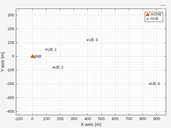
Create and configure UE nodes with different carrier aggregation capabilities by varying their distance from the gNB node. Position UE 1 and UE 2 close to the gNB node to enable support for all configured component carriers. Position UE 3 at a moderate distance to enable support for up to two component carriers. Position UE 4 farthest from the gNB, restricting it to the primary carrier.

uePositions = [100 50 1.5; 150 -80 1.5; 400 120 1.5; 850 -200 1.5];

% UE nodes with full CA capability
UEs_fullCA = nrUE(Name=["UE 1","UE 2"],Position=uePositions(1:2,:), ...
    NumComponentCarriers=numCCs,NumTransmitAntennas=2, ...
    NumReceiveAntennas=2,ReceiveGain=0,PHYModel=phyType);

% UE with up to 2 component carriers
UE_2CC = nrUE(Name="UE 3",Position=uePositions(3,:), ...
    NumComponentCarriers=min(2,numCCs),NumTransmitAntennas=2, ...
    NumReceiveAntennas=2,ReceiveGain=0,PHYModel=phyType);

% UE with single carrier
UE_1CC = nrUE(Name="UE 4",Position=uePositions(4,:), ...
    NumTransmitAntennas=2,NumReceiveAntennas=2, ...
    ReceiveGain=0,PHYModel=phyType);

UEs = [UEs_fullCA UE_2CC UE_1CC];

Connect all UE nodes to the gNB node on the primary carrier and enable full buffer traffic.

connectUE(gNB,UEs,FullBufferTraffic="on");

Activate the secondary carriers on the UE nodes that support carrier aggregation. UE 1 and UE 2 activate all secondary carriers. UE 3 activates one secondary carrier because it supports two component carriers in total.

% When numCCs=2, UE 3 has the same CA capability as UE 1 and UE 2
addSecondaryCarrierOnUE(gNB,UEs_fullCA,ccConfig(2:end));
addSecondaryCarrierOnUE(gNB,UE_2CC,ccConfig(2));

Add the gNB and UE nodes to the network simulator.

addNodes(networkSimulator,gNB)
addNodes(networkSimulator,UEs)

Create the CDL channels between the gNB and UE nodes. Create an N-by-N array of link-level channels, where N represents the number of nodes in the simulation. An element at index (i,j) contains the channel instance from node i to node j. An empty element at index (i,j) indicates the absence of a channel from node i to node j where i and j represent the node IDs.

In this example, each non-empty element contains a dictionary that is indexed by carrier frequency and has a separate nrCDLChannel instance for each component carrier. Carriers for the same link share the same carrier-independent properties, such as antenna geometry and delay profile. Each carrier has its own carrier-specific properties, such as carrier frequency, sample rate, maximum Doppler shift, and seed.

Create a custom channel model by using the per-carrier channels and add it to the network simulator.

c = physconst("LightSpeed");                  % Speed of light in m/s
vUE = 3*1000/3600;                            % UE speed in m/s (3 kmph)
fc = ccConfig(1).CarrierFrequency(1);         % First carrier frequency in Hz
fdMax = (vUE)/c*fc;                           % Maximum Doppler shift in Hz
channelConfig = struct(DelayProfile="CDL-C",DelaySpread=300e-9,MaximumDopplerShift=fdMax);
channels = hNRCreateCDLChannels(channelConfig,gNB,UEs);
% Create a custom channel model using the multi-carriers channels and
% install to the simulator. Network simulator applies the channel to a
% packet in transit before passing it to the receiver.
channel = hNRCustomChannelModel(channels, struct(PHYModel=phyType));
addChannelModel(networkSimulator,@channel.applyChannelModel)

Log scheduling and PHY information by setting the enableTraces flag to true.

enableTraces = true;

Create scheduling and PHY loggers.

if enableTraces
    % Create an object to log scheduler traces
    simSchedulingLogger = helperNRSchedulingLogger(numFrameSimulation,gNB,UEs,CarrierID=1:numCCs);
    % Create an object to log for PHY traces
    simPhyLogger = helperNRPhyLogger(numFrameSimulation,gNB,UEs,CarrierID=1:numCCs);
end

Set the metric refresh rate. A value of 10 updates the plots for every 100 ms of simulation time.

metricsRefreshRate = 10; % Updates plots every 100 milliseconds, as per the 1 second simulation time

Create the metrics visualizer.

metricsVisualizer = helperNRMetricsVisualizer(gNB,UEs, ...
    RefreshRate=metricsRefreshRate,PlotSchedulerMetrics=true, ...
    PlotPhyMetrics=true,PlotCDFMetrics=false);

Specify the name of the MAT file for the simulation logs. You can use these logs to analyze the simulation.

if enableTraces
    simulationLogFile = "simulationLogs"; % For logging the simulation traces
end

Display the network topology.

networkVisualizer = wirelessNetworkViewer;
addNodes(networkVisualizer,gNB)
addNodes(networkVisualizer,UEs)

Run the simulation for the specified number of frames.

% Calculate the simulation duration (in seconds)
simulationTime = numFrameSimulation * 1e-2;
% Run the simulation
run(networkSimulator,simulationTime);

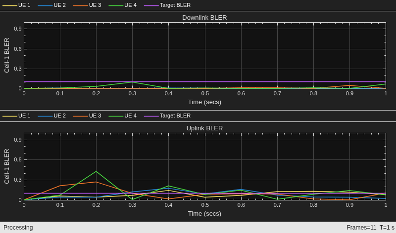
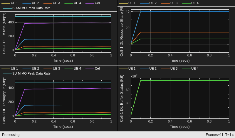
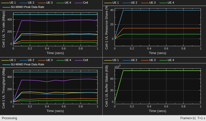
This example includes various runtime visualizations. The scheduler metrics plot shows per-UE throughput and buffer status. The PHY metrics plot shows the block error rates. The throughput plot shows the impact of carrier aggregation on the throughput of each UE. UE 1 and UE 2 achieve the highest throughput because their aggregate bandwidth is the largest. UE 3 which has fewer component carriers achieves moderate throughput. UE 4 which operates only on the primary carrier, achieves the lowest throughput since it does not benefit from carrier aggregation.

For more information about the runtime visualizations, see Simulation Visualizations.

Compute Key Performance Indicators

Display the performance indicators. The displayPerformanceIndicators function displays performance indicators for the DL and UL, including the achieved data rate, the achieved spectral efficiency, and the block error rate for the UE nodes. The calculated peak values follow 3GPP TR 37.910. This function aggregates metrics across all the configured component carriers. The function computes achieved data rate as the sum of per-carrier data rates, computes the spectral efficiency over the total aggregated bandwidth and computes the BLER as the average across carriers.

displayPerformanceIndicators(metricsVisualizer)

Peak UL throughput: 477.79 Mbps
Achieved cell UL throughput: 348.62 Mbps
Achieved UL throughput for each UE: [148.38        133.65         47.12         19.47]
Peak UL spectral efficiency: 11.94 bits/s/Hz
Achieved UL spectral efficiency for cell: 8.72 bits/s/Hz 
Block error rate for each UE in the UL direction: [0.086        0.08       0.097       0.125]

Peak DL throughput: 477.79 Mbps
Achieved cell DL throughput: 384.46 Mbps
Achieved DL throughput for each UE: [155.35        154.72         54.06         20.33]
Peak DL spectral efficiency: 11.94 bits/s/Hz
Achieved DL spectral efficiency for cell: 9.61 bits/s/Hz
Block error rate for each UE in the DL direction: [0       0.002       0.007       0.021]

Read per-node statistics.

gNBStats = statistics(gNB);
ueStats = statistics(UEs);

Analyze the Simulation Logs

Save the simulation logs in a MAT file. Open the MAT file to load DLTimeStepLogs, ULTimeStepLogs, SchedulingAssignmentLogs, PhyReceptionLogs in the workspace.

if enableTraces
    simulationLogs = cell(1,1);
    if gNB.DuplexMode == "FDD"
        logInfo = struct(DLTimeStepLogs=[],ULTimeStepLogs=[], ...
            SchedulingAssignmentLogs=[],PhyReceptionLogs=[]);
        [logInfo.DLTimeStepLogs,logInfo.ULTimeStepLogs] = getSchedulingLogs(simSchedulingLogger);
    else % TDD
        logInfo = struct(TimeStepLogs=[],SchedulingAssignmentLogs=[],PhyReceptionLogs=[]);
        logInfo.TimeStepLogs = getSchedulingLogs(simSchedulingLogger);
    end
    % Obtain the scheduling assignments log
    logInfo.SchedulingAssignmentLogs = getGrantLogs(simSchedulingLogger);
    % Obtain the Phy reception logs
    logInfo.PhyReceptionLogs = getReceptionLogs(simPhyLogger);
    simulationLogs{1} = logInfo;
    % Save simulation logs in a MAT-file
    save(simulationLogFile,"simulationLogs")
end

When you set enableTraces to true, the example stores the three simulation logs in MAT file for post-simulation analysis. The MAT file simulationLogFile contains the time step logs, the scheduling assignment logs, and the PHY reception logs.

For information about the log fields and their formats, see the NR Cell Performance Evaluation with MIMO example.

Further Exploration

Try running the example with these modifications to explore different aspects of carrier aggregation performance:

Supporting Functions

The example uses these helper functions: