NR FDD Scheduling Performance Evaluation

Introduction

To assign DL and UL resources, this example uses a round robin scheduler. The scheduler takes resource allocation decisions based on these inputs: pending retransmissions, buffer status, and channel quality for the UEs.

This example models:

The control packets required are assumed to be sent out of band without the need of resources for transmission. The control packets are UL assignment, DL assignment, buffer status report (BSR), and PDSCH feedback.

Scenario simulation

Check if the Communications Toolbox Wireless Network Simulation Library support package is installed. If the support package is not installed, MATLAB® returns an error with a link to download and install the support package.

wirelessnetworkSupportPackageCheck

Create a wireless network simulator.

rng("default") % Reset the random number generator
numFrameSimulation = 50; % Simulation time in terms of number of 10 ms frames
networkSimulator = wirelessNetworkSimulator.init;

Create a gNB node. Specify the duplex mode, carrier frequency, channel bandwidth, subcarrier spacing, and receive gain of the node.

gNB = nrGNB(DuplexMode="FDD",CarrierFrequency=2.6e9,ChannelBandwidth=30e6,SubcarrierSpacing=15e3,ReceiveGain=11);

To set the scheduler parameters Scheduler and ResourceAllocationType, use the configureScheduler function. Set the value of Scheduler parameter to RoundRobin and ResourceAllocationType to 0. You can also set the value of Scheduler to ProportionalFair or BestCQI and ResourceAllocationType to 1.

configureScheduler(gNB,Scheduler="RoundRobin",ResourceAllocationType=0);

Create 4 UE nodes. Specify the name, position and receive gain of each UE node.

uePositions = [100 0 0; 250 0 0; 700 0 0; 750 0 0];
ueNames = "UE-" + (1:size(uePositions,1));
UEs = nrUE(Name=ueNames,Position=uePositions,ReceiveGain=11);

Load the application configuration table containing these fields. Each row in the table represents one application and has these properties as columns.

load("NRFDDAppConfig.mat")
% Validate the host device type for the applications configured
validateattributes(AppConfig.HostDevice,{'numeric'},{"nonempty","integer",">=",0,"<=",1},"AppConfig.HostDevice", ...
    "HostDevice");

Load the RLC bearer configuration table. Each row in the table represents one RLC bearer and has these properties as columns.

load("NRFDDRLCChannelConfig.mat")

Create a set of RLC bearer configuration objects.

rlcBearerConfig = cell(1, length(UEs));
for rlcBearerInfoIdx = 1:size(RLCChannelConfig, 1)
    rlcBearerConfigStruct = table2struct(RLCChannelConfig(rlcBearerInfoIdx, 2:end));
    ueIdx = RLCChannelConfig.RNTI(rlcBearerInfoIdx);

    % Create an RLC bearer configuration object with the specified logical
    % channel ID
    rlcBearerObj = nrRLCBearerConfig(LogicalChannelID=rlcBearerConfigStruct.LogicalChannelID);
    % Set the other properties of the configuration object with specified values
    rlcBearerObj.LogicalChannelGroup = rlcBearerConfigStruct.LogicalChannelGroup;
    rlcBearerObj.SNFieldLength = rlcBearerConfigStruct.SNFieldLength;
    rlcBearerObj.BufferSize = rlcBearerConfigStruct.BufferSize;
    rlcBearerObj.ReassemblyTimer=rlcBearerConfigStruct.ReassemblyTimer;
    rlcBearerObj.Priority=rlcBearerConfigStruct.Priority;
    rlcBearerObj.PrioritizedBitRate=rlcBearerConfigStruct.PrioritizedBitRate;
    rlcBearerObj.BucketSizeDuration=rlcBearerConfigStruct.BucketSizeDuration;
    rlcBearerObj.RLCEntityType=rlcBearerConfigStruct.RLCEntityType;

    rlcBearerConfig{ueIdx} = [rlcBearerConfig{ueIdx} rlcBearerObj];
end

Connect the UE nodes to the gNB node using the connectUE object function. Specify the RLC bearer configuration for establishing an RLC bearer between the gNB node and each UE node, and set the buffer status report (BSR) periodicity to 5 (in number of subframes). For more information about BSR, see Communication Between gNB and UE Nodes.

for ueIdx = 1:length(UEs)
    connectUE(gNB,UEs(ueIdx),BSRPeriodicity=5,RLCBearerConfig=rlcBearerConfig{ueIdx})
end

Set the periodic DL and UL application traffic pattern for UEs.

for appIdx = 1:size(AppConfig,1)
    
    % Create an object for On-Off network traffic pattern
    app = networkTrafficOnOff(PacketSize=AppConfig.PacketSize(appIdx),GeneratePacket=true, ...
            OnTime=numFrameSimulation/100,OffTime=0,DataRate=AppConfig.DataRate(appIdx));

    if AppConfig.HostDevice(appIdx) == 0
        % Add traffic pattern that generates traffic on downlink
        addTrafficSource(gNB,app,DestinationNode=UEs(AppConfig.RNTI(appIdx)),LogicalChannelID=AppConfig.LogicalChannelID(appIdx))
    else
        % Add traffic pattern that generates traffic on uplink
        addTrafficSource(UEs(AppConfig.RNTI(appIdx)),app,LogicalChannelID=AppConfig.LogicalChannelID(appIdx))
    end
end

Add gNB node and UE nodes to the network simulator.

addNodes(networkSimulator,gNB)
addNodes(networkSimulator,UEs)

Set the enableTraces to true to log the traces. If the enableTraces is set to false, then traces are not logged in the simulation. To speed up the simulation, set the enableTraces to false.

enableTraces = true;

The cqiVisualization and rbVisualization parameters control the display of the CQI visualization and the RB assignment visualization respectively. By default, these plots are enabled. You can disable them by setting the respective flags to false.

cqiVisualization = true;
rbVisualization = true;

Set up RLC logger and scheduling logger.

if enableTraces
    % Create an object for RLC traces logging
    simRLCLogger = helperNRRLCLogger(numFrameSimulation,gNB,UEs);
    % Create an object for scheduler traces logging
    simSchedulingLogger = helperNRSchedulingLogger(numFrameSimulation,gNB,UEs);
    % Create an object for CQI and RB grid visualization
    gridVisualizer = helperNRGridVisualizer(numFrameSimulation,gNB,UEs,CQIGridVisualization=cqiVisualization, ...
        ResourceGridVisualization=rbVisualization,SchedulingLogger=simSchedulingLogger);
end

The example updates the metrics plots periodically. Set the number of updates during the simulation.

numMetricsSteps = 20;

Set up metric visualizer.

metricsVisualizer = helperNRMetricsVisualizer(gNB,UEs,NumMetricsSteps=numMetricsSteps, ...
    PlotSchedulerMetrics=true,PlotRLCMetrics=true);

Write the logs to MAT-files. The example uses these logs for post-simulation analysis and visualization.

simulationLogFile = "simulationLogs"; % For logging the simulation traces

Run the simulation for the specified numFrameSimulation frames.

% Calculate the simulation duration (in seconds)
simulationTime = numFrameSimulation*1e-2;
% Run the simulation
run(networkSimulator,simulationTime)

Read per-node stats.

gNBStats = statistics(gNB);
ueStats = statistics(UEs);

At the end of the simulation, the achieved value for system performance indicators is compared to their theoretical peak values (considering zero overheads). Performance indicators displayed are achieved data rate (UL and DL), achieved spectral efficiency (UL and DL), and block error rate (BLER) observed for UEs (UL and DL). The peak values are calculated as per 3GPP TR 37.910.

displayPerformanceIndicators(metricsVisualizer)

Peak UL Throughput: 199.08 Mbps. Achieved Cell UL Throughput: 121.95 Mbps
Achieved UL Throughput for each UE: [46.25        17.48         39.8        18.42]
Peak UL spectral efficiency: 6.64 bits/s/Hz. Achieved UL spectral efficiency for cell: 4.07 bits/s/Hz 
Peak DL Throughput: 199.08 Mbps. Achieved Cell DL Throughput: 131.47 Mbps
Achieved DL Throughput for each UE: [45.96         16.4        48.64        20.47]
Peak DL spectral efficiency: 6.64 bits/s/Hz. Achieved DL spectral efficiency for cell: 4.38 bits/s/Hz

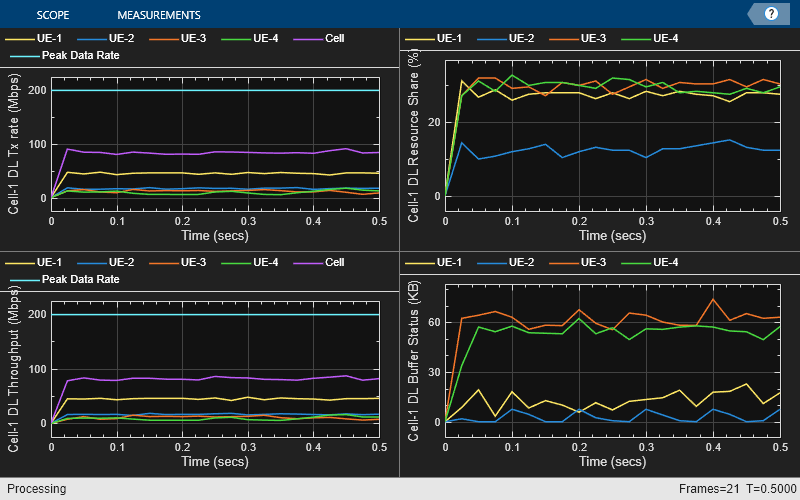
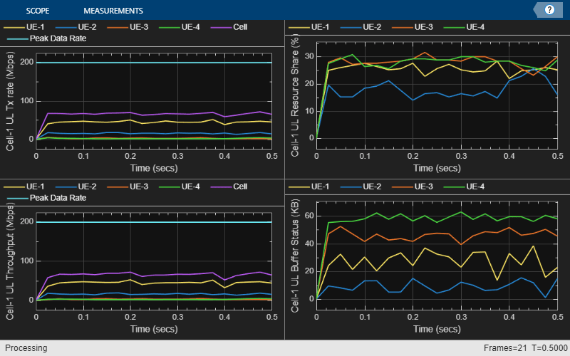
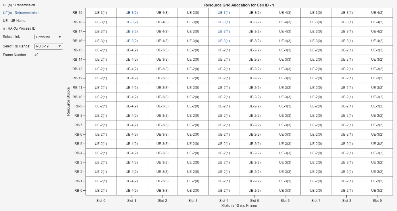
Simulation Visualization

The run-time visualization shown are:

Simulation Logs

The simulation logs are saved in MAT-files for post-simulation analysis. The per time step logs, scheduling assignment logs, and RLC logs are saved in the MAT-file simulationLogFile. After the simulation, open the file to load DLTimeStepLogs, ULTimeStepLogs, SchedulingAssignmentLogs, RLCLogs in the workspace.

Time step logs: For more information on the time step log format, see NR Cell Performance Evaluation with MIMO.

Scheduling assignment logs: For more information on the scheduling log format, see NR Cell Performance Evaluation with MIMO.

RLC logs: Each row in the RLC logs represents a slot and contains this information:

Each row of the UE and gNB RLC statistics table represents a logical channel of a UE and contains:

Save the simulation logs in a MAT file.

if enableTraces
    simulationLogs = cell(1,1);
    if gNB.DuplexMode == "FDD"
        logInfo = struct("DLTimeStepLogs",[],"ULTimeStepLogs",[],"SchedulingAssignmentLogs",[],"RLCLogs",[]);
        [logInfo.DLTimeStepLogs,logInfo.ULTimeStepLogs] = getSchedulingLogs(simSchedulingLogger);
    else % TDD
        logInfo = struct("TimeStepLogs",[],"SchedulingAssignmentLogs",[],"RLCLogs",[]);
        logInfo.TimeStepLogs = getSchedulingLogs(simSchedulingLogger);
    end
    % Get the scheduling assignments log
    logInfo.SchedulingAssignmentLogs = getGrantLogs(simSchedulingLogger);
    % Get the RLC logs
    logInfo.RLCLogs = getRLCLogs(simRLCLogger);
    % Save simulation logs in a MAT-file
    simulationLogs{1} = logInfo;
    save(simulationLogFile,"simulationLogs")
end

Further Exploration

Try running the example with these modifications.

TDD modeling

Explore TDD modeling by setting the DuplexMode property of the gNB object to "TDD". You can also customize the DL-UL slot pattern configuration for TDD by using the DLULConfigTDD property of the nrGNB object.

Full buffer traffic modeling

Consider using the full buffer traffic model instead of custom traffic models in this example. For more information on the workflow, see the NRFDDSchedulingPerformanceEvaluationWithFullBuffer.m script. This script evaluates the effect of scheduling algorithms (RR, PF, and Best CQI) on cell throughput for a simulation duration of 100 frames. The empirical cumulative distribution function (ECDF) plots demonstrate the evaluation results of RR, PF, and Best CQI scheduling algorithms. The Best CQI scheduling algorithm obtains a significant cell throughput gain in the UL and DL directions because it prioritizes the UEs with the best channel quality. The RR scheduling algorithm, on the other hand, obtains poor cell throughput because it prioritizes only fairness in scheduling. You can achieve a compromise between the RR and BestCQI scheduling algorithms when you use the PF scheduling algorithm.

Appendix

The example uses these helper classes: