Marine Navigation Using Planetary Ephemerides

This example uses:

This example shows how to perform celestial navigation of a marine vessel using the planetary ephemerides and an Earth-Centered Inertial to Earth-Centered Earth-Fixed (ECI to ECEF) transformation.

This example uses the Mapping Toolbox™. You must also download data for the example using the aeroDataPackage function.

This example uses the route followed by the 1947 expedition across the Pacific Ocean Kon-Tiki. The expedition, led by Thor Heyerdahl, aimed to prove the theory that the Polynesian islands were populated by people from South America in pre-Columbian times. The expedition took 101 days and sailed from the port of Callao, Peru, to the Raroia atoll, French Polynesia.

Notes: This example loosely recreates the expedition route. It takes some liberties to show the planetary ephemerides and ECI to ECEF transformation simply.

Load Vessel Track

Load the astKonTikiData.mat file. It contains the ship trajectory, velocity, and course for this example. This file stores the latitude and longitude for the different track points in the variables "lat" and "long", respectively. The variables contain enough data for one track point per day from the port of Callao to the Raroia atoll. This file also stores values for each day's vessel velocity in knots per day "V" and course in deg "T".

load astKonTikiData

Create an Observation Structure

The nautical reduction process is a series of steps that a navigator follows to determine the latitude and longitude of the vessel. It is based on the theory described in The American Practical Navigator[1], the Nautical Almanac[2], and the Explanatory Supplement to the Astronomical Almanac[3]. The process uses observational data obtained from a sextant, clock, compass, and navigational charts. It returns the intercept (p) and true azimuth (Z) for each of the observed objects. This example uses an observation structure array, obs, to contain the observational data. The fields for the structure array are:

h: Height of eye level of the observer, in m.
IC: Sextant's index correction, in deg.
P: Local ambient pressure, in mb.
T: Local temperature, in C.
year: Local year at the time of the observation.
month: Local month at the time of the observation.
day: Local day at the time of the observation.
hour: Local hour at the time of the observation.
UTC: Coordinated Universal Time for the observation, represented as a six element vector with year, month, day, hour, minutes, and seconds.
Hs: Sextant altitude of the celestial object above the horizon, in deg.
object: Celestial object used for the measurement (i.e., Jupiter, Neptune, Saturn, etc).
latitude: Estimated latitude of the vessel at the time of the observation, in deg.
longitude: Estimated longitude of the vessel at the time of the observation, in deg.
declination: Declination of the celestial object, in deg.
altitude: Distance from the surface of the Earth to the celestial object, in km.
GHA: Greenwich Hour Angle, which is the angle in degrees of the celestial object relative to the Greenwich meridian.

For simplicity, assume that all measurements are taken at the same location in the boat, with the same sextant, at the same ambient temperature and pressure:

obs.h = 4; 
obs.IC = 0; 
obs.P = 982;
obs.T = 15;

The expedition departed on April 28, 1947. As a result, initialize the structure for the observation for this date:

obs.year = 1947;
obs.month = 4; 
obs.day = 28;

Initialize Dead Reckoning Process for Navigation

To start the dead reckoning process, define the initial conditions for the position of the vessel. Store the latitude for a fixed solution for the latitude and longitude in the latFix and longFix variables, respectively. In this example, for the first fix location, use the latitude and longitude of Callao, Peru.

longFix = zeros(size(long));
latFix = zeros(size(lat));
longFix(1) = long(1);
latFix(1) = lat(1);

Daily Dead Reckoning

For this example, assume that a fix is obtained daily using the observational data. Therefore, this example uses a "for loop" for each observation. The variable m acts as a counter representing every elapsed day since the departure from the port.

for m = 1:size(lat,1)-1

Increment the day and make day adjustments for the months of June and April, both of which have only 30 days.

    obs.day = obs.day + 1;
    [obs.month,obs.day] = astHelperDayCheck(obs.year,obs.month,obs.day);

Actual Latitude and Longitude

Extract the vessel actual position for each day from the track points loaded earlier. The example uses this value to calculate the local time zone and the position of the selected planets in the sky.

    longActual = long(m+1);
    latActual = lat(m+1);

Planet Selection

Select the planets for observation if they are visible to the vessel for the given latitude and longitude. The following code uses precalculated data.

    if longActual>-90
        obs.object = {'Saturn';'Neptune'};
    elseif longActual<=-90 && longActual>-95
        obs.object = {'Saturn';'Neptune';'Jupiter'}; 
    elseif longActual<=-95
        obs.object = {'Neptune';'Jupiter'};
    end

UTC Time Calculation

Adjust local time to UTC depending on the assumed longitude. For this example, assume that all observations are taken at the same time every day at 8 p.m. local time.

    obs.hour = 20;

For the dead reckoning process, update the observation structure with the estimate of the current location. In this case, the location is estimated using the previous fix, the vessel's velocity V, and course T.

    obs.longitude = longFix(m)+(1/60)*V(m)*sind(T(m))/cosd(latFix(m));
    obs.latitude = latFix(m)+(1/60)*V(m)*cosd(T(m));

Adjust the local time to UTC using the helper function astHelperLongitudeHour. This function adjusts the UTC observation time depending on the estimated longitude of the vessel.

    obs.UTC = astHelperLongitudeHour(obs);

Sextant Altitude Calculation

For each of the planets, the astHelperNauticalCalculation helper function calculates the sextant measurement that the crew in the Kon-Tiki would have measured. This function models the actual behavior of the planets, while compensating for the local conditions. This function uses the planetary ephemeris and the ECI to ECEF transformation matrix. The analysis doesn't include planetary aberration, gravitational light deflection, and aberration of light phenomena.

    obs.Hs = astHelperNauticalCalculation(obs,latActual,longActual);

Calculate Position

The following calculations replace the use of the nautical almanac. They include the use of the planetary ephemerides and the ECI to ECEF transformation matrix.

Initialize declination, Greenwich Hour Angle (GHA), and altitude for the observed object.

    obs.declination = zeros(size(obs.Hs));
    obs.GHA = zeros(size(obs.Hs));
    obs.altitude = zeros(size(obs.Hs));

Calculate the modified Julian date for the measurement time.

    mjd = mjuliandate(obs.UTC);

Calculate the difference between UT1 and UTC:

    dUT1 = deltaUT1(mjd,'Action','None');

Calculate the ECI to ECEF transformation matrix using the values of TAI-UTC (dAT) from the U.S. Naval Observatory.

    dAT = 1.4228180;
    TM = dcmeci2ecef('IAU-76/FK5',obs.UTC,dAT,dUT1);

Calculate Julian date for Terrestrial Time to approximate the Barycentric Dynamical Time.

    jdTT = juliandate(obs.UTC)+(dAT+32.184)/86400;

Calculate declination, Greenwich Hour Angle, and altitude for each of the celestial objects.

    for k =1:length(obs.object)

Calculate the ECI position for every planet.

        posECI = planetEphemeris(jdTT,'Earth',obs.object{k},'405','km');

Calculate the ECEF position of every planet.

        posECEF = TM*posECI';

Calculate the Greenwich Hour Angle (GHA) and declination using the ECEF position.

        obs.GHA(k) = -atan2d(posECEF(2),posECEF(1));
        obs.declination(k) = atan2d(posECEF(3),sqrt(posECEF(1)^2 + ...
            posECEF(2)^2));

Calculate the distance from the surface of the Earth to the center of the planet using the ECEF to LLA transformation function.

        posLLA = ecef2lla(1000*posECEF');
        obs.altitude(k) = posLLA(3);
 
    end

Sight Reduction for Planetary Objects

Reduce sight for each of the planets specified in the observation structure array.

    [p,Z] = astHelperNauticalReduction(obs);

Calculate the increments to the latitude and longitude from the last fix for the current fix using these equations. These equations are based on the Nautical Almanac.

    Ap = sum(cosd(Z).^2);
    Bp = sum(cosd(Z).*sind(Z));
    Cp = sum(sind(Z).^2);
    Dp = sum(p.*cosd(Z));
    Ep = sum(p.*sind(Z));
    Gp = Ap*Cp-Bp^2;

Calculate the increments for latitude and longitude according to the reduction.

    deltaLongFix = (Ap*Ep-Bp*Dp)/(Gp*cosd(latFix(m)));
    deltaLatFix = (Cp*Dp-Bp*Ep)/Gp;

After the increments for the latitude and longitude are calculated, add them to the estimated location, obtaining the fix for the time of observation.

    longFix(m+1) = obs.longitude + deltaLongFix;
    latFix(m+1) = obs.latitude + deltaLatFix;

end

Navigation Solution Visualization

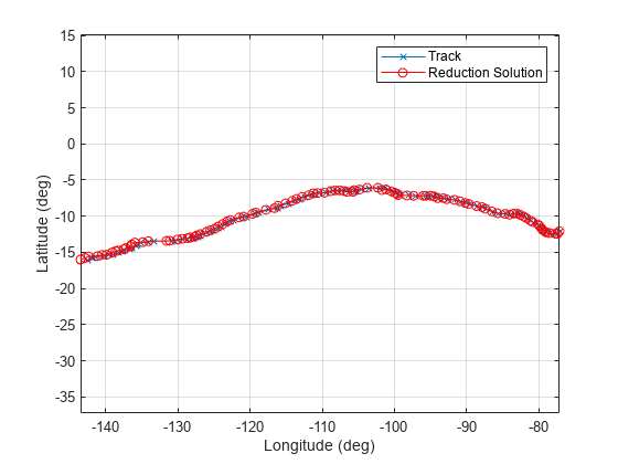
This figure shows the actual track and sight reduction solutions.

astHelperVisualization(long,lat,longFix,latFix,'Plot')

Figure contains an axes object. The axes object with xlabel Longitude (deg), ylabel Latitude (deg) contains 2 objects of type line. These objects represent Track, Reduction Solution.

Figure contains 2 axes objects. Axes object 1 with title Relative error in Latitude and Longitude, ylabel Error in Longitude (deg) contains an object of type line. Axes object 2 with xlabel Date [mm/dd], ylabel Error in Latitude (deg) contains an object of type line.

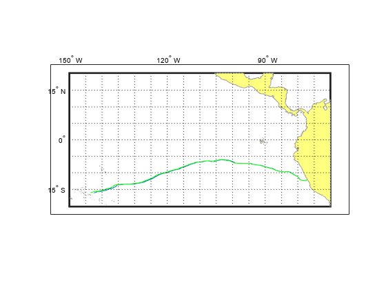
You can use the Mapping Toolbox to obtain a more detailed graph depicting the sight reduction solutions with the American continent and French Polynesia.

if builtin('license','test','MAP_Toolbox')
    astHelperVisualization(long,lat,longFix,latFix,'Map')
end

Figure contains an axes object. The axes object contains 544 objects of type patch, line, text.

The relative error in longitude and latitude is accumulated as the vessel sails from Callao to Raroia. This error is due to small errors in the measurement of the sextant altitude. For June 9th, the reduction method calculates a true azimuth (Z) for Neptune and Jupiter. The true azimuths for Neptune and Jupiter are close to 180 deg apart. This difference causes a small peak in the relative error. This error, however, is still within the reduction method error boundaries.

References

[1] Bowditch, N. The American Practical Navigator. National Geospatial Intelligence Agency, 2012.

[2] United Kingdom Hydrographic Office. Nautical Almanac 2012 Commercial Edition. Paradise Publications, Inc. 2011.

[3] Urban, Sean E. and P. Kenneth Seidelmann. Explanatory Supplement to the Astronomical Almanac. 3rd Ed., University Science Books, 2013.

[4] United States Naval Observatory.