Modeling Station-Keeping Using Impulsive Maneuvers

R2026b

This example demonstrates the planning of a sequence of impulsive maneuvers for orbital station-keeping using a bounded in-plane relative motion trajectory. Station-keeping involves maintaining the position of a spacecraft (the active spacecraft) in close proximity of another spacecraft (the target spacecraft). The approach considered here combines an initial phasing maneuver with periodic correction maneuvers to produce a closed relative trajectory. Between these maneuvers, the spacecraft motion is governed by two‑body orbital dynamics. While this motion follows fundamental orbital mechanics, the trajectory, when expressed in the target-centered frame, exhibits a distinctive teardrop-like geometry that remains entirely below the target spacecraft.

Assume that both the active and target spacecraft are in circular, coplanar orbits, with the active spacecraft initially at a slightly lower altitude than the target. In the absence of corrective maneuvers, the active spacecraft travels at a higher orbital velocity and will drift ahead of the target over time. To establish a bounded relative motion, a small retrograde delta-V is applied to initiate a phasing maneuver, causing the active spacecraft to fall behind the target.

Following this maneuver, the spacecraft evolves under nonlinear two-body dynamics, descending to a lower altitude and accelerating as gravitational potential energy is converted into kinetic energy. This natural evolution reduces the along-track separation and brings the spacecraft to a point directly below the target. At this location, the spacecraft possesses a nonzero radial velocity component directed downward when expressed in its local-vertical/local-horizontal (LVLH) frame.

A corrective impulsive maneuver is then applied to reverse this radial velocity component while leaving the tangential component unchanged. In the LVLH frame, this operation is equivalent to reflecting the velocity vector about the local horizontal plane. Because the magnitude of the velocity is preserved, the specific orbital energy remains unchanged; however, the direction of motion is altered, initiating an upward trajectory.

As the spacecraft ascends, kinetic energy is converted back into potential energy, reducing its speed as it returns toward its initial altitude. On completing the cycle, the spacecraft returns to the same geometric configuration with the same velocity state (relative to the initial phasing offset), enabling periodic repetition of the motion.

The resulting trajectory is a closed, periodic relative orbit maintained through discrete symmetry operations at the lowest point. Its projection in the target-centered frame forms a characteristic teardrop-shaped path that lies entirely below the target spacecraft. Periodic impulsive corrections applied at this point sustain the motion over successive cycles. The complete sequence is illustrated in the figure below.

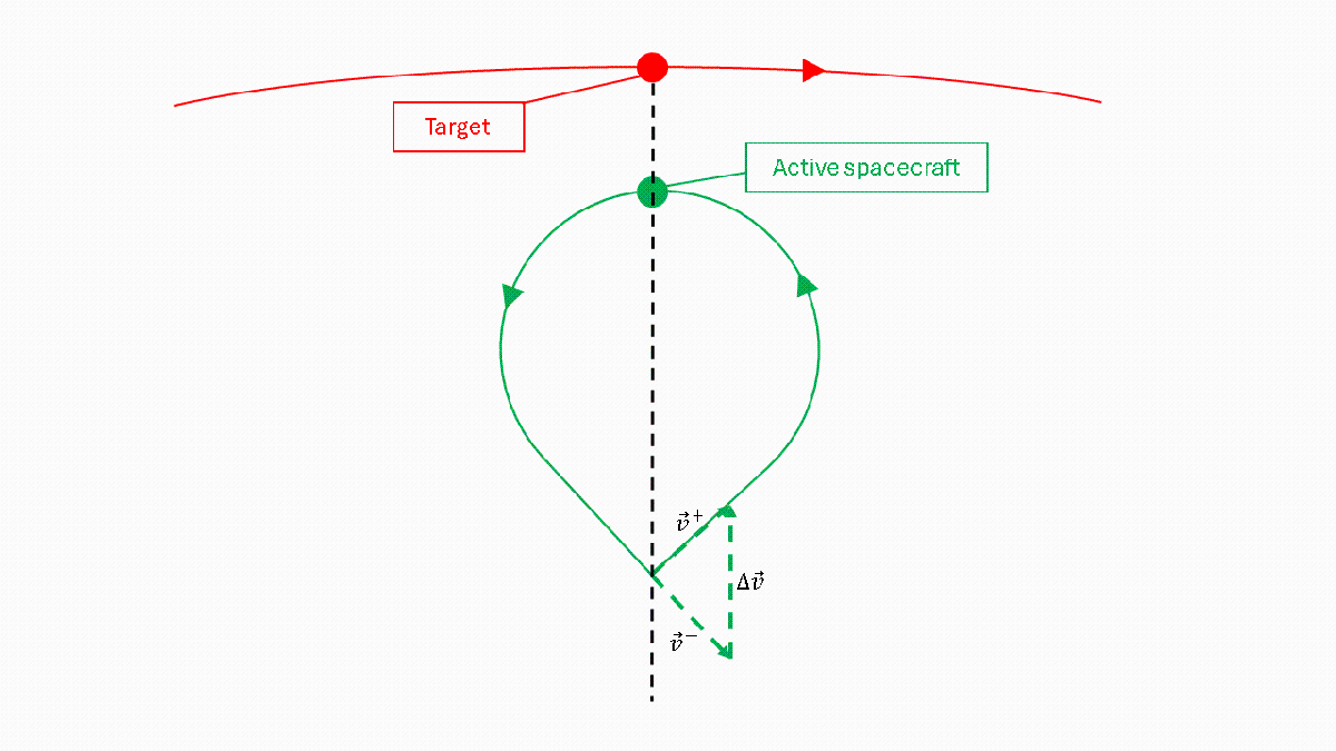
To quantify the cost of maintaining this motion, the total propellant expenditure associated with the sequence of impulsive maneuvers is evaluated. Each delta-V applied during the cycle contributes to the overall propulsion requirement, which can be translated into propellant mass using the Tsiolkovsky rocket equation. By aggregating the delta-V contributions from each cycle, the analysis provides an estimate of the propellant required to sustain the teardrop-shaped station-keeping trajectory over the desired operational duration.

Set Up Satellite Scenario

Create a satellite scenario object with StartTime, StopTime and SampleTime set to May 20, 2026, 12:00 AM UTC, May 20, 2026, 6:00 AM UTC and 10 seconds respectively.

startTime = datetime(2026, ... % Year
    5, ...                     % Month
    20);                       % Day
stopTime = datetime(2026, ...  % Year
    5, ...                     % Month
    20, ...                    % Day
    6, ...                     % Hour
    0, ...                     % Minute
    0);                        % Second
sampleTime = 10;               % s
sc = satelliteScenario(startTime,stopTime,sampleTime);

Add the target spacecraft to the scenario. Place it in a circular equatorial orbit of radius 10,000 km. Set OrbitPropagator to "two-body-keplerian".

semiMajorAxisTarget = 10000000;    % m
eccentricity = 0;
inclination = 0;                   % deg
rightAscensionofAscendingNode = 0; % deg
argumentOfPeriapsis = 0;           % deg
trueAnomaly = 0;                   % deg
target = satellite(sc, ...
    semiMajorAxisTarget, ...
    eccentricity, ...
    inclination, ...
    rightAscensionofAscendingNode, ...
    argumentOfPeriapsis, ...
    trueAnomaly, ...
    Name = "Target", ...
    OrbitPropagator="two-body-keplerian");

Add the active spacecraft 10 meters below the target in a coplanar circular orbit. Set OrbitPropagator to "two-body-keplerian".

semiMajorAxisActive = semiMajorAxisTarget - 10; % m
active = satellite(sc, ...
    semiMajorAxisActive, ...
    eccentricity, ...
    inclination, ...
    rightAscensionofAscendingNode, ...
    argumentOfPeriapsis, ...
    trueAnomaly, ...
    Name = "Active", ...
    OrbitPropagator="two-body-keplerian");

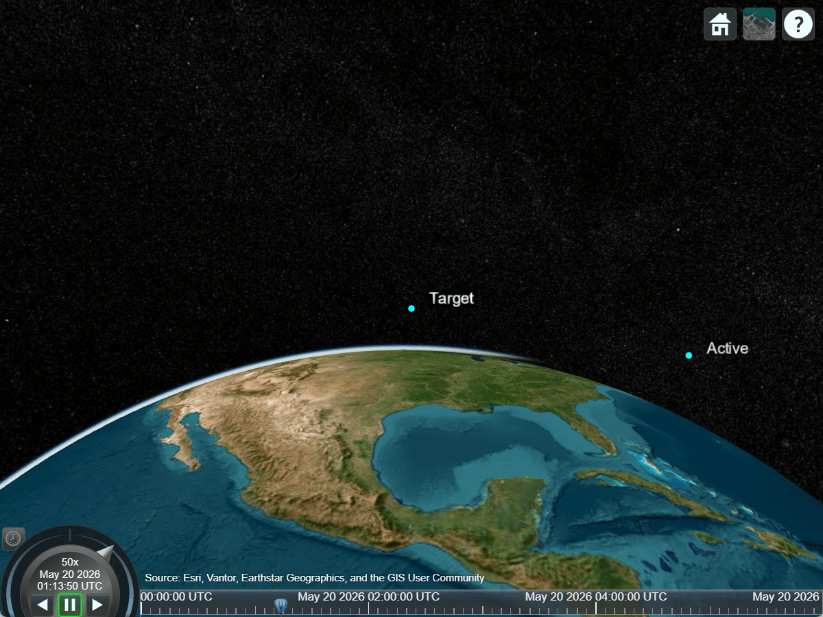
Play the scenario in the Satellite Scenario Viewer and observe the relative motion. Notice that the active spacecraft is in a lower circular orbit, which results in a shorter orbital period than the target spacecraft. Because station-keeping maneuvers have not yet been applied, the active spacecraft moves at a higher orbital velocity and gradually drifts ahead of the target.

viewer = satelliteScenarioViewer(sc);
hide([target.Orbit active.Orbit]);
play(sc);
camtarget(viewer,target);

Plan and Execute Station-Keeping Maneuvers

This section introduces the station-keeping maneuvers required to establish the bounded relative motion. The objective is to place the active spacecraft on a teardrop-shaped trajectory with respect to the target. To initiate this motion, a one-time retrograde delta-V is applied as part of a phasing maneuver. This reduces the instantaneous velocity of the active spacecraft below the local circular speed, placing it on an orbit with lower energy and causing it to initially lag behind the target.

The maneuver is defined in the velocity-normal-binormal (VNB) frame, where the x-axis is aligned with the instantaneous velocity vector in the International Celestial Reference Frame (ICRF) frame, the y-axis is aligned with the orbit angular momentum vector, and the z-axis completes the right-handed coordinate triad. The required delta-V is applied purely in the negative velocity direction and is expressed as:

$Δ {v_{}^{\to}}_{V N B} = (\begin{array}{c} - Δ v \\ 0 \\ 0 \end{array})$

where $Δ v > 0$ denotes the magnitude of the retrograde impulse. For this example set $Δ v$ to 0.02 m/s.

Time = startTime;
DeltaV = [-0.02;0;0]'; % m/s
CoordinateFrame = "vnb";
Name = "Phasing maneuver";
maneuver = timetable(Time,DeltaV,CoordinateFrame,Name);
impulsiveManeuver(active,Insert=maneuver);

Play the scenario again in the Satellite Scenario Viewer and observe the relative motion.

play(sc);
camtarget(viewer,target);

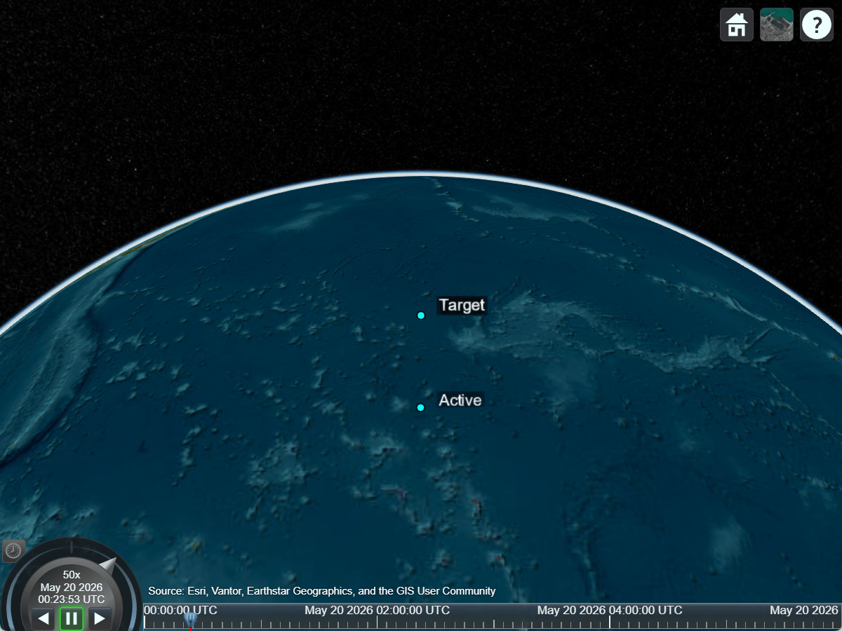
Immediately following the maneuver, the reduced velocity results in a trajectory for which the gravitational acceleration exceeds that required for a circular orbit at the current radius. As a result, the active spacecraft begins to descend to a lower altitude. During this descending phase, gravitational potential energy is converted into kinetic energy, causing the spacecraft to accelerate and progressively reduce its along-track separation with the target as it moves along the lower branch of the trajectory.

To maintain the desired periodic motion, a corrective impulsive maneuver must be applied at a specific point along this descending–ascending path. This point corresponds to the configuration in which the active spacecraft passes directly below the target, where the trajectory transitions from descending toward ascending. Identifying the precise instant at which this configuration occurs requires monitoring the relative geometry between the active and target spacecraft throughout the motion.

To determine this maneuver location, the scenario is advanced in a controlled manner. Specifically, the AutoSimulate property of the satellite scenario is set to false, allowing the simulation to be stepped forward manually through discrete time samples.

sc.AutoSimulate = false;

Manually advance the scenario time step in a loop using advance. At each time step, evaluate the relative geometry between the active and target spacecraft using their position vectors in ICRF. Let ${r_{}^{\to}}_{a}$ and ${r_{}^{\to}}_{t}$ denote the position vectors of the active and target spacecraft, respectively. The angular separation between the two spacecraft is computed as:

$θ = \cos^{- 1} (\frac{{r_{}^{\to}}_{t} \cdot ({r_{}^{\to}}_{t} - {r_{}^{\to}}_{a})}{‖ {r_{}^{\to}}_{t} ‖ ‖ {r_{}^{\to}}_{t} - {r_{}^{\to}}_{a} ‖})$

The bottom of the teardrop trajectory corresponds to the configuration in which the active spacecraft lies directly below the target, which ideally occurs when $θ = 0$ . However, because the simulation advances in fixed time increments, this condition is not satisfied exactly at a sampled time. Instead, the maneuver point is identified by detecting when the angular separation transitions through zero and selecting the first time sample immediately after this crossing.

By stepping through the scenario and evaluating the angular separation at each time step, the time corresponding to the bottom of the trajectory can be approximated. The corrective impulsive maneuver is then applied at this discrete time, ensuring that the trajectory closely enforces the intended symmetry and maintains the bounded teardrop-shaped motion.

At this identified maneuver point, the required delta-V is computed to reverse the radial component of the velocity of the active spacecraft while preserving the tangential component. This corrective action is expressed in the local-vertical/local-horizontal (LVLH) frame centered on the active spacecraft. In this frame, the x-axis is aligned with the spacecraft position vector (defined as the vector from the center of the celestial body to the spacecraft), the z-axis is aligned with the orbit angular momentum vector, and the y-axis completes the right-handed coordinate triad. The outward radial direction is therefore parallel to the LVLH x-axis.

Let ${v_{}^{\to}}_{a}$ denote the instantaneous ICRF velocity of the active spacecraft. The corrective maneuver is then defined in the LVLH frame as:

$Δ {v_{}^{\to}}_{L V L H} = - 2 ({v_{}^{\to}}_{a} \cdot {x_{}^{ˆ}}_{L V L H}) {x_{}^{ˆ}}_{L V L H}$

This expression computes the impulsive correction by projecting the velocity onto the LVLH negative x-axis (nadir direction) and applying a delta-V with twice the magnitude of this projected component, directed along the x-axis. In effect, this operation reverses the x-component of the velocity while leaving the remaining components unchanged.

As a result, the maneuver preserves the specific orbital energy and redirects the spacecraft from a descending trajectory to an ascending one, thereby maintaining the symmetric, closed teardrop-shaped motion.

Before executing the above logic programmatically, close the Satellite Scenario Viewer to improve performance during code execution, particularly when stepping through the scenario time samples. The viewer can then be relaunched after the simulation for playback.

delete(viewer);

Initialize variable that stores the angle between the position vector of the target and the relative position vector of the target with respect to the active spacecraft.

previousAngle = 0;

Initialize a counter for tracking the number of correction maneuvers executed at the bottom of the teardrop.

maneuverCount = 0;

Advance the simulation time step and apply the logic for executing the corrective maneuvers.

while advance(sc)
    % Retrieve the position and velocity histories of the spacecraft up to
    % the current simulation time.
    [positionHistoryTarget,velocityHistoryTarget] = states(target);
    [positionHistoryActive,velocityHistoryActive] = states(active);

    % Get the position and velocity at the current time step.
    positionTarget = positionHistoryTarget(:,end);
    velocityTarget = velocityHistoryTarget(:,end);
    positionActive = positionHistoryActive(:,end);
    velocityActive = velocityHistoryActive(:,end);

    % Get the position of the target with respect to the active spacecraft.
    relativePositionTarget = positionTarget - positionActive;

    % Get the angle between the position vector of target and relative
    % position of target with respect to the active spacecraft.
    ang = real(acos(dot(positionTarget,relativePositionTarget)/ ...
        (norm(positionTarget)*norm(relativePositionTarget))));

    % Determine how much the angle changed when compared to the previous
    % time step.
    deltaAngle = ang - previousAngle;

The active spacecraft is at the bottom of the teardrop when the angle is 0 degrees and the spacecraft is overtaking the target. However, because satellite scenario uses fixed time steps and does not support zero-crossing detection, you cannot determine the exact instant when the active spacecraft is at the bottom of the teardrop. Therefore, the algorithm attempts to find the closest time step after the spacecraft crosses the bottom.

To identify this condition, verify that:

The angle is 0 degrees, or the angle has increased compared to the previous time step. The reasoning is that just before crossing the bottom, the angle decreases. After crossing the bottom, the angle starts increasing. Additionally, you only check for an increasing angle when the angle is less than 0.01 radians so that the check is performed only when the spacecraft is in the vicinity of the bottom (or top) of the teardrop.

    isAngleZeroOrCrossingZero = ...
        (ang == 0 || (deltaAngle > 0 && abs(ang) < 0.01));

2. The angular velocity of the active spacecraft is greater than that of the target. This check is required because (1) is true at both top

and bottom of the teardrop. However, at the top, the target starts

leading the active, while at the bottom, the active starts leading

the target.

    isActiveAngularVelocityGreaterThanTarget = ...
        ((norm(velocityActive)/norm(positionActive)) > ...
        (norm(velocityTarget)/norm(positionTarget)));

3. The active spacecraft must be descending.

    isDescending = dot(velocityActive,positionActive) < 0;

    if isAngleZeroOrCrossingZero && ...
            isActiveAngularVelocityGreaterThanTarget && ...
            isDescending
        % Active spacecraft is at the bottom of the teardrop.

        % Define the LVLH x-axis as the unit vector parallel to the
        % position vector of the active spacecraft.
        xLVLH = positionActive/norm(positionActive);

        % The delta-V is defined as a vector that is anti-parallel to twice
        % the projection of the velocity vector of the active spacecraft on
        % the LVLH x-axis.
        deltaV = [-2*dot(velocityActive,xLVLH);0;0]; % m/s

        % Execute the maneuver.
        maneuverCount = maneuverCount + 1;
        maneuverName = ...
            "Station-keeping correction maneuver " + maneuverCount;
        impulsiveManeuver(active,deltaV, ...
            CoordinateFrame="lvlh", ...
            Name=maneuverName);
    end

    % Update the previous angle.
    previousAngle = ang;
end

Visualize Scenario

Launch the satellite scenario viewer again and hide the orbits. Play the scenario and observe the relative motion. At the initial time, the phasing maneuver is applied to initiate the teardrop trajectory.

viewer = satelliteScenarioViewer(sc);
hide([target.Orbit active.Orbit]);
play(sc);
camtarget(viewer,target);

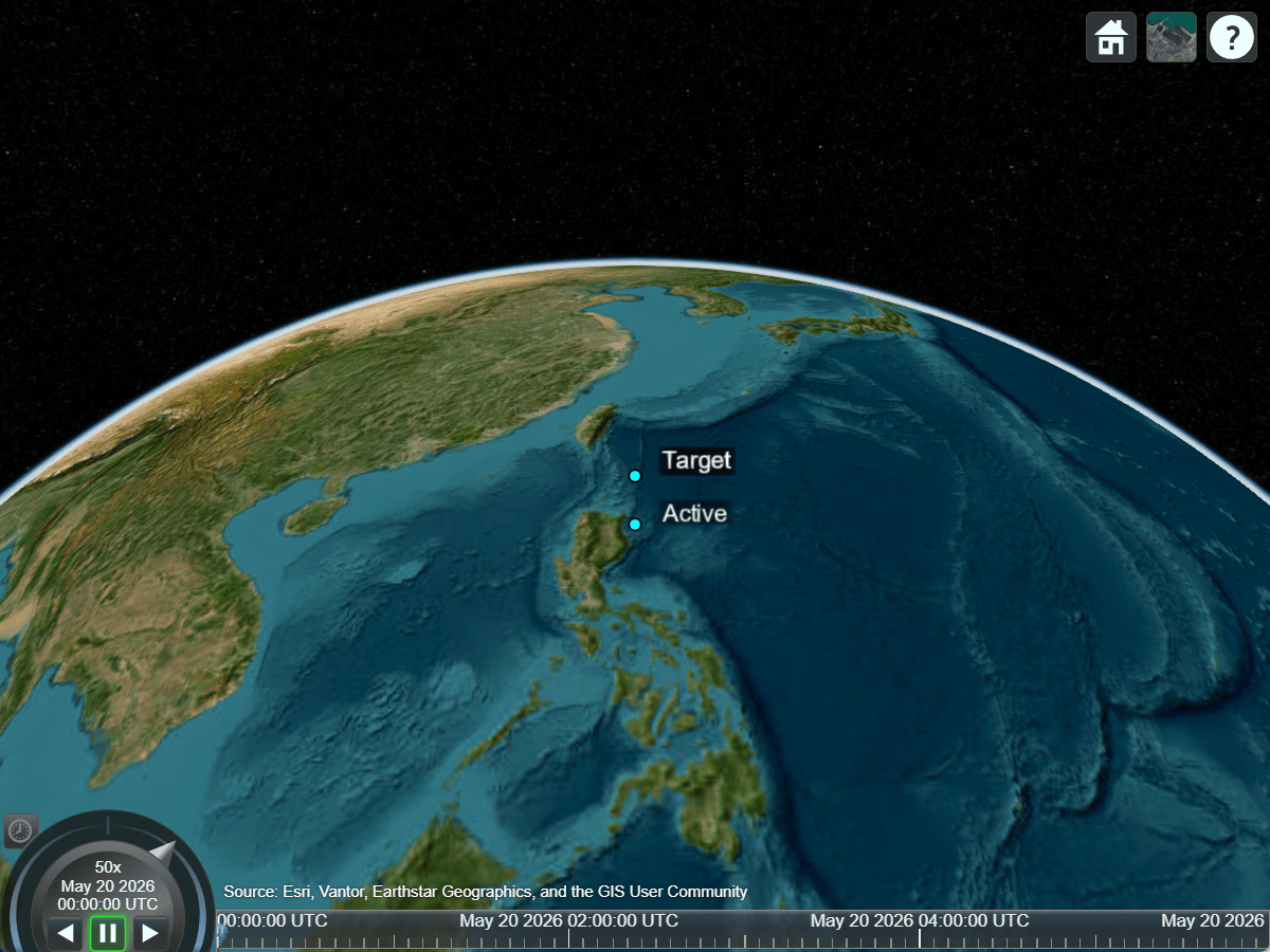
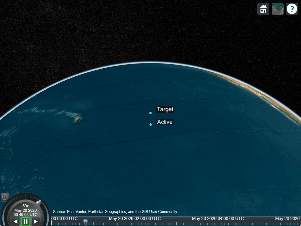
As the active spacecraft evolves along the descending branch, it reaches the point directly below the target, where the station-keeping correction maneuver is executed. This maneuver reverses the radial component of the velocity, redirecting the motion along the ascending branch of the trajectory.

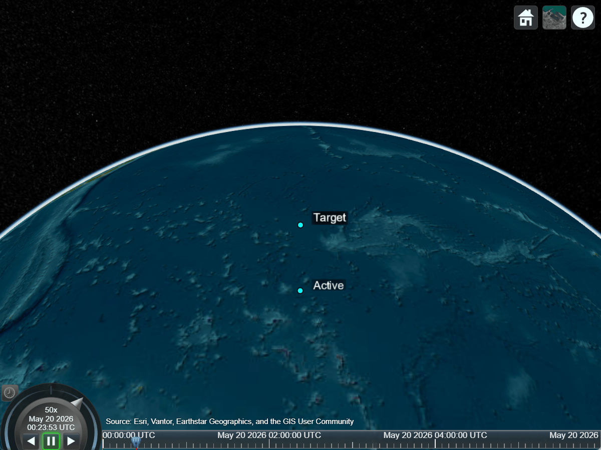
The spacecraft subsequently returns to its original relative position with respect to the target, completing one cycle of the motion. The process then repeats, resulting in a sustained teardrop-shaped relative orbit.

Visualize Relative Motion on MATLAB Plot

To complement the Satellite Scenario Viewer playback, generate an animated MATLAB plot of the motion of the active spacecraft relative to the target in the LVLH frame. The relative position is expressed in target-centered LVLH coordinates to provide an intuitive view of the in-plane motion, and the plot is animated over time to show how the teardrop-shaped path is established and maintained by the impulsive maneuvers.

Get the ICRF position history of the active spacecraft.

[positionActive,~,time] = states(active);

Get the ICRF position and velocity history of the target spacecraft.

[positionTarget, velocityTarget] = states(target);

Construct a history of direction cosine matrices relating ICRF to the target-centered LVLH frame.

x = positionTarget./vecnorm(positionTarget);
z = cross(positionTarget,velocityTarget);
z = z./vecnorm(z);
y = cross(z,x);
numTimeSamples = numel(time);
icrfTolvlh = zeros(3,3,numTimeSamples);
icrfTolvlh(1,:,:) = x;
icrfTolvlh(2,:,:) = y;
icrfTolvlh(3,:,:) = z;

Get the relative position of active spacecraft with respect to target spacecraft in target-centered LVLH frame.

relativePosition = positionActive - positionTarget;
relativePositionLVLH = reshape( ...
    pagemtimes(icrfTolvlh,reshape(relativePosition,3,1,[])),3,[]);

Plot the relative trajectory of the target. For visualization purposes, the plot axes are defined as remapped versions of the LVLH axes so that the teardrop trajectory appears in the desired orientation. The plot axes and LVLH axes are related as follows: the plot x-axis corresponds to the LVLH y-axis, the plot y-axis corresponds to the LVLH z-axis, and the plot z-axis corresponds to the LVLH x-axis.

pTraj = plot3(relativePositionLVLH(2,:),relativePositionLVLH(3,:),relativePositionLVLH(1,:));
hold on
axis equal

Plot the markers for the active and target spacecraft.

pTarget = plot3(0,0,0,'m.',MarkerSize=20);
pActive = plot3(relativePositionLVLH(2,1), ...
    relativePositionLVLH(3,1), ...
    relativePositionLVLH(1,1), ...
    'b.',MarkerSize=20);
hold off

Set the axis limits.

xlim(xlim);
ylim(ylim);
zlim(zlim);

Add plot legend and define the axis labels. The axis labels shown in the plot reflect the corresponding LVLH directions rather than the plot coordinate names. That is, the plot x-axis is labeled y, the plot y-axis is labeled z, and the plot z-axis is labeled x.

legend(["Relative trajectory of active", "Target", "Active"]);
xlabel("y, m")
ylabel("z, m")
zlabel("x, m")
drawnow

Update the target spacecraft trajectory history and marker in a loop to animate the plot.

for idx = 1:10:numel(time)
    set(pTraj, ...
        XData=relativePositionLVLH(2,1:idx), ...
        YData=relativePositionLVLH(3,1:idx), ...
        ZData=relativePositionLVLH(1,1:idx));
    set(pActive, ...
        XData=relativePositionLVLH(2,idx), ...
        YData=relativePositionLVLH(3,idx), ...
        ZData=relativePositionLVLH(1,idx));
    drawnow;
end

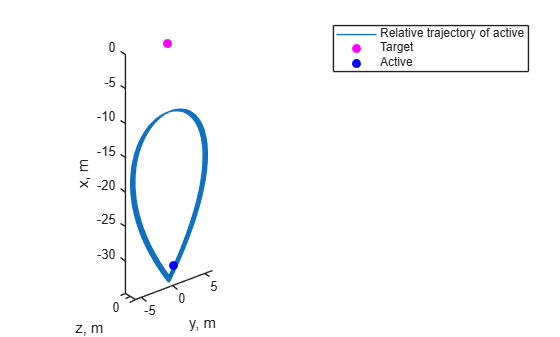
Figure contains an axes object. The axes object with xlabel y, m, ylabel z, m contains 3 objects of type line. One or more of the lines displays its values using only markers These objects represent Relative trajectory of active, Target, Active.

From the plot and inspection of the relativePosition data, the maximum distance of the active spacecraft from the target is observed to be 34.7 m.

max(vecnorm(relativePosition))

ans = 
34.7468

Estimate Total Propellant Budget for Phasing and Station-Keeping Maneuvers

To quantify the propellant requirement for the maneuver sequence, obtain a timetable of the maneuvers that were scheduled.

maneuvers = active.ImpulsiveManeuvers

maneuvers = 9×4 timetable
            Time                             Name                                   DeltaV                 CoordinateFrame    ReferenceCelestialBody
    ____________________    _______________________________________    ________________________________    _______________    ______________________

    20-May-2026 00:00:00    "Phasing maneuver"                            -0.02           0           0        "vnb"                 "Earth"        
    20-May-2026 00:24:10    "Station-keeping correction maneuver 1"    0.063427           0           0        "lvlh"                "Earth"        
    20-May-2026 01:12:00    "Station-keeping correction maneuver 2"    0.062492           0           0        "lvlh"                "Earth"        
    20-May-2026 01:59:50    "Station-keeping correction maneuver 3"    0.063427           0           0        "lvlh"                "Earth"        
    20-May-2026 02:47:50    "Station-keeping correction maneuver 4"    0.062806           0           0        "lvlh"                "Earth"        
    20-May-2026 03:35:40    "Station-keeping correction maneuver 5"    0.063117           0           0        "lvlh"                "Earth"        
    20-May-2026 04:23:30    "Station-keeping correction maneuver 6"    0.062805           0           0        "lvlh"                "Earth"        
    20-May-2026 05:11:30    "Station-keeping correction maneuver 7"    0.063427           0           0        "lvlh"                "Earth"        
    20-May-2026 05:59:20    "Station-keeping correction maneuver 8"    0.062492           0           0        "lvlh"                "Earth"        

	Get insights using Copilot

Compute the total mission $Δ v$ by aggregating the magnitudes of all impulsive deltaV maneuvers - both the initial phasing maneuver and these stationkeeping correction maneuvers.

deltaVMagnitude = sum(vecnorm(maneuvers.DeltaV'));

Use this total delta-V to estimate the propellant consumption by applying the Tsiolkovsky rocket equation, assuming a specific impulse ( $I_{s p}$ ) of 310 s and an initial spacecraft mass ( $m_{0}$ ) of 6,000 kg. The Tsiolkovsky rocket equation relates the initial mass and the final mass ( $m_{f}$ ) using the following equation:

$m_{f} = m_{0} e^{- (\frac{Δ v}{g_{0} I_{s p}})}$

where $g_{0}$ denotes the standard acceleration due to gravity at the surface of the Earth.

initialMass = 6000;    % kg
specificImpulse = 310; % s
g0 = 9.80665;          % m/s^2
finalMass = initialMass/exp(deltaVMagnitude/(g0*specificImpulse));

The total propellant consumed is the difference between the initial and final masses.

propellantConsumed = initialMass - finalMass

propellantConsumed = 
1.0341

Effect of Phasing Maneuver Delta-V on Trajectory and Propellant Budget

The magnitude of the initial phasing maneuver delta-V determines the characteristics of the resulting trajectory, including the maximum separation from the target, the total number of maneuvers, and the overall propellant consumption.

For a reduced delta-V magnitude of 0.01 m/s, the maximum separation decreases to 11.83 m and the propellant consumption decreases to 0.55 kg. This reduction, however, requires a higher maneuver frequency, resulting in a total of 27 maneuvers over the same scenario duration.

In contrast, increasing the delta-V magnitude to 0.03 m/s leads to a larger maximum separation of 57.6 m and higher propellant consumption of 1.49 kg, while reducing the total number of maneuvers to 8.

These results highlight a fundamental tradeoff between propellant consumption and maneuver frequency, with larger delta-V values reducing operational complexity at the cost of increased separation and propellant usage.

Modeling Station-Keeping Using Impulsive Maneuvers

Set Up Satellite Scenario

Plan and Execute Station-Keeping Maneuvers

Visualize Scenario

Visualize Relative Motion on MATLAB Plot

Estimate Total Propellant Budget for Phasing and Station-Keeping Maneuvers

Effect of Phasing Maneuver Delta-V on Trajectory and Propellant Budget

See Also

Objects

Functions

Topics