Analysis of Monopole Impedance

Choose Frequency of Operation and Calculate Wavelength

Choose the operating frequency for the monopole and calculate the wavelength in free space at the frequency.

f = 400e6;
speedOfLight = physconst("lightspeed");
lambda = speedOfLight/f;

Select Physical Parameters of Monopole

The monopole is typically fed by a coaxial transmission line of characteristic impedance 50 ohm. Define the height of the monopole to be slightly less than quarter-wavelength [1], $$h/\lambda =0.236$$. The radius of the monopole also influences the impedance. Define the radius in terms of wavelength, $$a/\lambda =0.001588$$. The monopole model in the Antenna Toolbox ™ uses a metal strip. The width of the strip, w, is related to the radius, a, of an equivalent metal cylinder by $$w=4a$$ [2]. Choose a large ground plane by specifying the length and width of the ground plane to be twice the operating wavelength.

h_over_lambda = 0.236;
a_over_lambda = 0.001588;
h = h_over_lambda*lambda;
a = a_over_lambda*lambda;
w = cylinder2strip(a);
gpL = 2*lambda;
gpW = 2*lambda;

Create and Modify Monopole

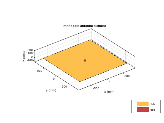
Create a monopole antenna and modify its properties to match the design parameters.

mp = monopole;
mp.Height = h;
mp.Width = w;
mp.GroundPlaneLength = gpL;
mp.GroundPlaneWidth = gpW;
figure
show(mp)

Calculate Baseline Impedance

Calculate and store the impedance and the number of triangles in the mesh when using the default mesh size.

Zbaseline = impedance(mp,f);
meshdata = mesh(mp);
Nbaseline = meshdata.NumTriangles;

Meshing Parameter Variation

You can evaluate the accuracy of the results by changing resolution of a triangular surface mesh. The triangular surface mesh implies a discretization of the surface geometry into small planar triangles. All antenna surfaces in the Antenna Toolbox ™ are discretized into triangles. To specify the resolution of the mesh, provide the size of the maximum edge length, i.e. the longest side of a triangle among all triangles in the mesh, prior to analysis. Alternatively, define a range of values for the maximum edge length.

maxEdgeLength = gpL./(2:2:16);

Set up Analysis Parameters

Create arrays to save impedance, relative change in impedance and the size of the mesh.

m = length(maxEdgeLength);
Zin = zeros(1,m);
numTri = zeros(1,m);
tolValue = 0.05.*ones(1,m);
tolCheck = nan*ones(1,m);
Ztemp = Zin(1);

Calculate Impedance Variation

For each value of the maximum edge length, update the mesh, calculate the impedance at the operating frequency and the number of triangles in the mesh. Save the impedance and number of triangles in the mesh for the convergence analysis. Finally, calculate the relative change in the impedance between subsequent mesh refinement steps.

for i = 1:m
    mesh(mp,MaxEdgeLength=maxEdgeLength(i));
    Zin(i) = impedance(mp,f);
    meshdata = mesh(mp);
    numTri(i) = meshdata.NumTriangles;
    Zchange = abs((Zin(i)-Ztemp)/Zin(i));
    Ztemp = Zin(i);
    tolCheck(i) = Zchange;
end

Impedance of Monopole on Finer Meshes

Plot the input impedance at the operating frequency for each mesh update. Observe that the baseline values of the resistance, $$R_{in}$$ and reactance, $$X_{in}$$ are (for the default mesh),

$\begin{array}{l}{R}_{in}\approx \\ \text{37}\Omega \end{array}$, $\begin{array}{l}{X}_{in}\approx \\ \text{2}\Omega \end{array}$.

The result published in [1] for the case $$a/\lambda =.001588$$, $$l/\lambda =0.236$$

is

$$R_{in}=36.82$$ $$\Omega$$, $$X_{in}=0$$ $$\Omega$$

Our result matches the resistance and suggests that a weak inductive component is present as well. The circled values for resistance and reactance are the results obtained for the default baseline mesh. Note, that the results of [1] cited above are related to cylindrical monopoles; they take into account the effect of a gap between the inner conductor and the outer conductor of the coaxial transmission line. Our geometrical model approximates the cylindrical monopole with a rectangular strip and does not account for the gap in the groundplane.

figure;
plot(numTri,real(Zin),'*-',LineWidth=2)
hold on
plot(numTri,imag(Zin),'r*-',LineWidth=2)
hold on
plot(Nbaseline,real(Zbaseline),'o',MarkerSize=10)
plot(Nbaseline,imag(Zbaseline),'ro',MarkerSize=10)
axis([min(numTri),max(numTri),-10*abs(round(min(imag(Zin)))),...
      1.5*floor(max(max(real(Zin),max(imag(Zin)))))])
grid on
xlabel("Number of triangles")
ylabel("Input Impedance Z_i_n - \Omega")
legend("R_i_n","X_i_n")
title("Monopole Impedance vs. No. of Triangles in Mesh")

References

[1] R. Elliott, 'Antenna Theory & Design,' Chapter 8, p.353, Wiley-IEEE Press, 2003.

[2] C. A. Balanis, 'Antenna Theory. Analysis and Design,' p.514, Wiley, New York, 3rd Edition, 2005.