Optimize and Analyze Antenna

Since R2026a

This example uses:

This example shows how to optimize the geometry of a horn antenna using the training cost-reduced surrogate-model-assisted differential evolution for antenna synthesis (TR-SADEA) optimizer, along with AI-based analysis of resonant frequency, bandwidth, beamwidth, and peak radiation. TR-SADEA is an enhanced version of the surrogate-model-assisted differential evolution for antenna synthesis (SADEA) algorithm, designed to further reduce the computational cost associated with surrogate model training. The objective of this example is to maximize gain and bandwidth while ensuring that the resonant frequency remains close to the design frequency and the beamwidth stays below 30 degrees.

By integrating AI-based analysis into the TR-SADEA optimization workflow, the overall optimization process becomes significantly faster than traditional EM solver-based optimization. This enables rapid exploration of the design space and identification of high-performance antenna configurations in a fraction of time.

Set Up and Run Optimization

Design the horn antenna for a 10 GHz operating frequency. This antenna has five tunable geometric parameters: Width, Height, FlareLength, FlareHeight, and FeedHeight. Each parameter can vary within ±15% of its default value. In addition, subject the design to a linear geometric constraint to ensure geometric feasibility during optimization:

$(- H e i g h t + F e e d H e i g h t \leq 0)$

ant = horn;
f = 10e9;
antAI = design(ant,f,ForAI=true);

L = antAI.defaultTunableParameters.FlareLength;
W = antAI.defaultTunableParameters.Width;
H = antAI.defaultTunableParameters.Height;
Flh = antAI.defaultTunableParameters.FlareHeight;
Fdh = antAI.defaultTunableParameters.FeedHeight;

N = 5; % Design variables

Define the lower and upper bounds for each parameter (±15%). Create TR-SADEA optimizer object with bounds. Specify the evaluation function and enable optimization logs.

Bounds = [0.85*W 0.85*H 0.85*L 0.85*Flh 0.85*Fdh;1.15*W 1.15*H 1.15*L 1.15*Flh 1.15*Fdh];
s = OptimizerTRSADEA(Bounds);
s.CustomEvaluationFunction = @customEval;
s.EnableLog(true);

Define the geometric constraints using the coefficients of linear inequality.

A = [0 -1 0 0 1]; % coefficients for ['Width','Height','FlareLength','FlareHeight','FeedHeight']
b = 0;
constraintsStructure.A = A;
constraintsStructure.b = b;
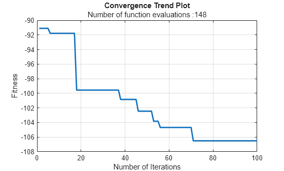
s.GeometricConstraints = constraintsStructure;

Run the optimization for 100 iterations and view the convergence trend plot.

tic
s.optimize(100);
topt = toc

topt = 
48.2652

figure
s.showConvergenceTrend

Figure contains an axes object. The axes object with title Convergence Trend Plot, xlabel Number of Iterations, ylabel Fitness contains an object of type line.

Get the optimization results.

bestData = s.getBestMemberData;

Define Custom Evaluation Function

The customEval function defines the fitness criteria used during optimization. It combines multiple performance objectives and applies penalties to guide the optimizer toward high-quality antenna designs. Because the TR‑SADEA optimizer minimizes the fitness value, it converts maximization objectives into minimization objectives.

Optimization Objectives

The function evaluates the antenna based on the following goals:

Maximize peak gain
Maximize bandwidth
Minimize deviation from the target resonant frequency (10 GHz)
Minimize beamwidth

Penalty Conditions

The function imposes penalties when the evaluated antenna violates any of the following conditions:

Gain < 15.5 dB
Resonant frequency deviation > 0.2%
Bandwidth < 10 MHz
Beamwidth > 30°

All objectives and penalties combine into a single scalar fitness value. Because the TR‑SADEA optimizer minimizes this value:

For maximization objectives, multiply the objective's contribution by –1 so that a larger physical value produces a smaller (and therefore better) fitness value.
For minimization objectives, add a positive weight to the objective's contribution, because lower values already indicate better performance.

This process ensures that all objectives are handled consistently by the optimizer.

function fitness = customEval(var)
f = 10e9;  % Target design frequency (Hz)
ant = horn;
antAI = design(ant, f, ForAI=true);

% Assign design variables to antenna geometry
antAI.Width       = var(1);
antAI.Height      = var(2);
antAI.FlareLength = var(3);
antAI.FlareHeight = var(4);
antAI.FeedHeight  = var(5);

try
    % Evaluate antenna performance
    gain = peakRadiation(antAI, f);        
    fr = resonantFrequency(antAI);         
    [bw, ~, ~, ~] = bandwidth(antAI);      
    bwth = beamwidth(antAI, f);            

    % Use azimuth beamwidth if multiple values are returned
    if numel(bwth) > 1
        bwth = bwth(1);
    end

    % Penalty for gain
    if gain < 15.5
        pen1 = -gain;
    else
        pen1 = -5*gain;  % Reward higher gain more strongly
    end

    % Calculate deviation from the target frequency
    deltaf = abs(fr-f)/f;

    % Penalty for frequency deviation
    if deltaf > 0.002
        pen2 = 1e2*deltaf;
    else
        pen2 = 0;
    end

    % Reward for bandwidth
    pen3 = -1*(bw/1e8);

    % Beamwidth penalty 
    if bwth < 30
        pen4 = 0.1*bwth;
    else
        pen4 = 10*bwth;
    end

    % Total fitness (lower is better)
    fitness = pen1 + pen2 + pen3 + pen4;

catch
    % In case of simulation failure, assign high penalty
    fitness = 1e6;
end
end

Analyze Optimized Antenna

Create an AI-based horn antenna (baseline) as well as an AI-based antenna with its tunable parameters set using the optimization results. Run the analysis on these antennas.

d = horn;
f = 10e9;
dAI = design(d,f,ForAI=true);

frAI_design = resonantFrequency(dAI);
[bwAI_design,~,~,~] = bandwidth(dAI);
pAI_design = peakRadiation(dAI,f);
bwthAI = beamwidth(dAI,f);
bwthAI_design = bwthAI(1);

dAI.Width = bestData.member(1);
dAI.Height = bestData.member(2);
dAI.FlareLength = bestData.member(3);
dAI.FlareHeight = bestData.member(4);
dAI.FeedHeight = bestData.member(5);

frAI_best = resonantFrequency(dAI);
[bwAI_best,~,~,~] = bandwidth(dAI);
pAI_best = peakRadiation(dAI,f);
bwthAI = beamwidth(antAI,f);
bwthAI_best = bwthAI(1);

Create a regular horn antenna from the AI-based antenna using the exportAntenna function. Run the EM-solver-based analysis on it, and compare the results with AI-based analysis.

antEm = exportAntenna(dAI);
freqR = linspace(0.7*f,1.5*f,51);
fr1 = resonantFrequency(antEm,freqR);
fr_Em = fr1(find(abs(f-fr1)==min(abs(f-fr1))));
bw_Em = bandwidth(antEm,freqR); 
bw_Em = max(bw_Em);
[bwp1_Em,angp1] = beamwidth(antEm,f,0,0:1:360);
[bwp2_Em,angp2] = beamwidth(antEm,f,0:1:360,0);
pg_Em = peakRadiation(antEm,f);

Create a table that compares the baseline antenna performance at the design frequency with the results from the two optimization approaches: AI-based analysis and EM-solver-based analysis.

designFreqRes = [frAI_design,bwAI_design,pAI_design,bwthAI_design]';
optAntAIRes = [frAI_best,bwAI_best,pAI_best,bwthAI_best]';
optAntEMRes = [fr_Em,bw_Em,pg_Em,bwp1_Em]';

t = table(designFreqRes,optAntAIRes,optAntEMRes,VariableNames=...
    ["DesignFrequencyResults","OptimizedAntennaAIAnalysis","OptimizedAntennaEMAnalysis"],...
    RowNames=["fres","bandwidth","peakRad","beamwidth"])

t=4×3 table
                 DesignFrequencyResults    OptimizedAntennaAIAnalysis    OptimizedAntennaEMAnalysis
                 ______________________    __________________________    __________________________

    fres               9.9009e+09                   1.037e+10                    1.0294e+10        
    bandwidth          2.2388e+09                  3.4754e+09                     3.047e+09        
    peakRad                 15.51                      15.611                        15.619        
    beamwidth              27.503                      27.503                            26

Optimize and Analyze Antenna

Set Up and Run Optimization

Define Custom Evaluation Function

Analyze Optimized Antenna

See Also

Objects

Functions

Topics