Wave Impedance

Open Live Script

This example will use an elementary dipole and loop antenna and analyze the wave impedance behavior of each radiator in space at a single frequency. The region of space around an antenna has been defined in a variety of ways. The most succinct description is using a 2-or 3-region model. One variation of the 2-region model uses the terms near-field and far-field to identify specific field mechanisms that are dominant. The 3-region model, splits the near-field into a transition zone, wherein a weakly radiative mechanism is at work. Other terms that have been used to describe these zones, include, quasistatic field, reactive field, non-radiative field, Fresnel region, induction zone etc. [1]. Pinning these regions down mathematically presents further challenges as observed with the variety of definitions available across different sources [1]. Understanding the regions around an antenna is critical for both an antenna engineer as well as an electromagnetic compatibility(EMC) engineer. The antenna engineer may want to perform near-field measurements and then compute the far-field pattern. To the EMC engineer, understanding the wave impedance is required for designing a shield with a particular impedance to keep interference out.

Create Electrically Short Dipole and Small Loop Antenna

For this analysis the frequency is 1 GHz. The length and circumference of the dipole and loop are selected so that they are electrically short at this frequency.

f = 1e9;
c = physconst('lightspeed');
lambda = c/f;
wavenumber = 2*pi/lambda;
d = dipole;
d.Length = lambda/20;
d.Width = lambda/400;
circumference = lambda/20;
r = circumference/(2*pi);
l = loopCircular;
l.Radius = r;
l.Thickness = circumference/200;

Create Nodal Points in Space to Calculate Fields

The wave impedance is defined in a broad sense as the ratio of the magnitudes of the total electric and magnetic field, respectively. The magnitude of a complex vector is defined to be the length of the real vector resulting from taking the modulus of each component of the original complex vector. To examine impedance behavior in space, choose a direction and vary the radial distance R from the antenna along this direction. The spherical coordinate system is used with azimuth and elevation angles fixed at (0,0) while R is varied in terms of wavelength. For selected antennas, the maximum radiation occurs in the azimuthal plane. The smallest value of R has to be greater than the structure dimensions, i.e. field computations are not done directly on the surface.

N = 1001;
az = zeros(1,N);
el = zeros(1,N);
R = linspace(0.1*lambda,10*lambda,N); 
x = R.*sind(90-el).*cosd(az);
y = R.*sind(90-el).*sind(az);
z = R.*cosd(90-el);
points = [x;y;z];

Calculate Electric and Magnetic Fields at Nodal Points

Since the antennas are electrically small at the frequency of 1 GHz, mesh the structure manually by specifying a maximum edge length. The surface mesh is a triangular discretization of the antenna geometry. Compute electric and magnetic field complex vectors.

md = mesh(d,'MaxEdgeLength',0.0003);
ml = mesh(l,'MaxEdgeLength',0.0003);

[Ed,Hd] = EHfields(d,f,points);
[El,Hl] = EHfields(l,f,points);

Total Electric and Magnetic Fields

The electric and magnetic field results from function EHfields is a 3-component complex vector. Calculate the resulting magnitudes of the electric and magnetic field component wise, respectively

Edmag = abs(Ed);
Hdmag = abs(Hd);

Elmag = abs(El);
Hlmag = abs(Hl);

% Calculate resultant E and H
Ed_rt = sqrt(Edmag(1,:).^2 + Edmag(2,:).^2 + Edmag(3,:).^2);
Hd_rt = sqrt(Hdmag(1,:).^2 + Hdmag(2,:).^2 + Hdmag(3,:).^2);

El_rt = sqrt(Elmag(1,:).^2 + Elmag(2,:).^2 + Elmag(3,:).^2);
Hl_rt = sqrt(Hlmag(1,:).^2 + Hlmag(2,:).^2 + Hlmag(3,:).^2);

Calculate Wave Impedance

The wave impedance can now be calculated at each of the predefined points in space as the ratio of the total electric field magnitude to the total magnetic field magnitude. Calculate this ratio for both the dipole antenna and the loop antenna.

ZE = Ed_rt./Hd_rt;
ZH = El_rt./Hl_rt;

Impedance of Free Space

The material properties of free space, the permittivity and permeability of vacuum, are used to define the free space impedance $η$ .

eps_0 = 8.854187817e-12;
mu_0 = 1.2566370614e-6;
eta = round(sqrt(mu_0/eps_0));

Plot Wave Impedance as a Function of Distance

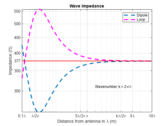
The behavior of wave impedance for both antennas is given on the same plot. The x-axis is the distance from the antenna in terms of $λ$ and the y-axis is the impedance measured in $Ω$ .

fig1 = figure;
loglog(R,ZE,'--','LineWidth',2.5)
hold on
loglog(R,ZH,'m--','LineWidth',2.5)
line(R,eta.*ones(size(ZE)),'Color','r','LineWidth',1.5);
textInfo = 'Wavenumber, k = 2\pi/\lambda';
text(0.4,310,textInfo,'FontSize',9)
ax1 = fig1.CurrentAxes;
ax1.XTickLabelMode = 'manual';
ax1.XLim = [min(R) max(R)];
ax1.XTick = sort([lambda/(2*pi) 5*lambda/(2*pi) lambda 1 5*lambda ax1.XLim]);
ax1.XTickLabel = {'0.1\lambda';'\lambda/2\pi';'5\lambda/2\pi'; '\lambda'; 'k\lambda/2\pi';'5\lambda';'10\lambda'};
ax1.YTickLabelMode = 'manual';
ax1.YTick = sort([ax1.YTick eta]);
ax1.YTickLabel = cellstr(num2str(ax1.YTick'));
xlabel('Distance from antenna in \lambda (m)')
ylabel('Impedance (\Omega)')
legend('Dipole','Loop')
title('Wave Impedance')
grid on

Figure contains an axes object. The axes object with title Wave Impedance, xlabel Distance from antenna in lambda blank (m), ylabel Impedance ( Omega ) contains 4 objects of type line, text. These objects represent Dipole, Loop.

Discussion

The plot of the wave impedance variation reveals several interesting aspects.

The wave impedance changes with distance from the antenna and shows opposing behaviors in the case of the dipole and the loop. The dipole, whose dominant radiation mechanism is via the electric field, shows a minima close to the radian sphere distance, $λ / 2 π$ , whilst the loop which can be thought of as a magnetic dipole shows a maxima in the impedance.
The region below the radian sphere distance, shows the first cross-over across 377 $Ω$ . This cross over occurs very close to the structure, and the quick divergence indicates that we are in the reactive near-field.
Beyond the radian sphere distance ( $λ / 2 π$ ), the wave impedance for the dipole and loop decreases and increases respectively. The impedance starts to converge towards the free space impedance value of $η = 377 Ω$ .
Even at a distance of 5 $λ / 2 π$ - $1 λ$ from the antennas, the wave impedance has not converged, implying that we are not yet in the far-field.
At a distance of $k λ / 2 π = 1$ and beyond, the values for wave impedance are very nearly equal to 377 $Ω$ . Beyond 10 $λ$ , the wave impedance stabilizes and the region of space can be termed as the far-field for these antennas at the frequency of 1GHz.
Note that the dependence on wavelength implies that these regions we have identified will change if the frequency is changed. Thus, the boundary will move in space.

Reference

[1] C. Capps, "Near Field or Far Field," EDN, August 16, 2001, pp. 95-102. Online at: http://m.eet.com/media/1140931/19213-150828.pdf