Loudspeaker Modeling with Simscape
This example shows how to model a dynamic loudspeaker using linear and nonlinear lumped element models.
Introduction to Loudspeaker Modeling
Dynamic loudspeaker drivers convert electrical signals into acoustic waves using electromagnetic energy to produce mechanical movements in a cone-shaped diaphragm. Therefore, three main domains must be represented in the model: electrical, mechanical, and acoustical, in addition to the bidirectional energy conversions between these.
A common linear model for a loudspeaker is to represent it as an electrical circuit, which is known as a lumped element model. The mechanical and acoustic effects are represented by electrical circuits that are mathematically equivalent models.
For the electrical model, the motor is composed of the voice coil and the magnet. The voice coil is driven by a voltage  and has a resistance
  and an inductance
  . These two parameters depend on the wire material, diameter, length, turn radius, number of turns, and other physical properties. The magnet also has an impact on the coil inductance because of the addition of a ferrous core.
The magnet creates a field in the gap with a flux density  . Multiplied by the wire length
  , this is known as the force factor
  . This is also the conversion factor between the electrical and mechanical domains, as there is a force
  applied to the voice coil, where
  is the electrical current applied at the input. Inversely, there is a voltage
  generated by
  which is analogous to the cone velocity. When converting the mechanical model to an electrical model, the coupling between them is represented by a gyrator, where velocity corresponds to the electrical current and force corresponds to the voltage.
For the mechanical model, lumped electrical components are used as analogues to mechanical properties such as mass and compliance. First, the inertia of the total moving mass (including the coil, cone, and dust cap) is analogous to the effect of an inductance  on varying electrical currents. Second, the stiffness of the suspension and spider is analogous to the effect of a capacitor
  . Thirdly, the mechanical loss in the suspension system is analogous to a resistor
  . This mechanical model forms a circuit with resonant frequency
  , which implies that the efficient frequency range of the driver depends on its mass.
For the acoustical model, the driver cone surface interface with the air is analogous to a transformer. The larger the cone is, the more mechanical energy is transformed to acoustic energy (at least for a given mass). An impedance  (formed by
  ,
,  and
and  ) models the radiation resistance for the front and the back of the cone. For a non-enclosed driver, this value is nonlinear but relatively small. An enclosed driver has a fixed amount of air, which creates a compliance modeled by a capacitor , and any air leaks (including a vent) will contribute to the resistance . For a vented enclosure, the mass of air moving in and out acts as an inductor .
For simplicity, the remainder of this example assumes a loudspeaker in free space, i.e. no enclosure ( ).
).
The equation for the electrical part of the model is:
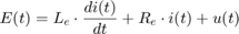
The equation for the mechanical part of the model is:
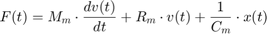
Where: 
The equations for a gyrator are:


Linear Loudspeaker Models
Using Simscape™, a loudspeaker can be modeled using a mixed-domain approach (mixing electrical and mechanical domains), or with a familiar model that converts the mechanical domain into the electrical domain.
First, implement the electrical model shown above, using a gyrator directly.
model = 'LinearGyrator';
open_system(model);
sim(model,1);

close_system(model,0)
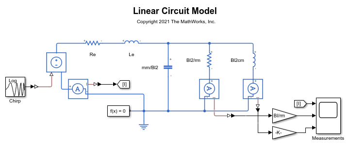
For analysis, the gyrator is often removed by rearranging the circuit topology and the elements values.
It can be shown that this circuit behaves the same as above with the following components:


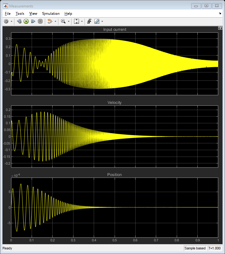
This simplified circuit produces the exact same results as before.
model = 'LinearCircuit';
open_system(model);
sim(model,1);

close_system(model,0)
Simscape™ also allows mixing electrical and mechanical elements, so the loudspeaker model can be simulated without any physical domain conversions. Again, the same results are obtained.
model = 'LinearMixedDomain';
open_system(model);
sim(model,1);

close_system(model,0)
Other elements can easily be added to this circuit model to account for a closed or vented enclosure.
Adding DSP to a Physical Model
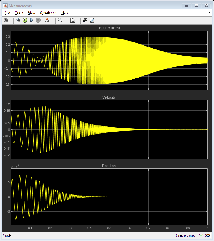
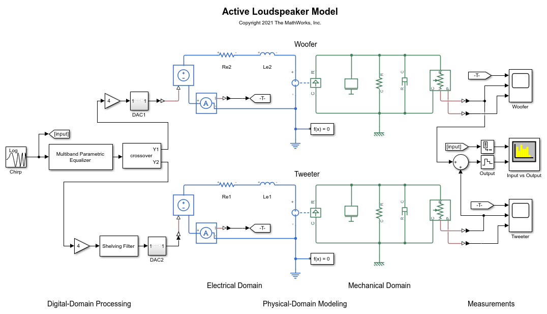
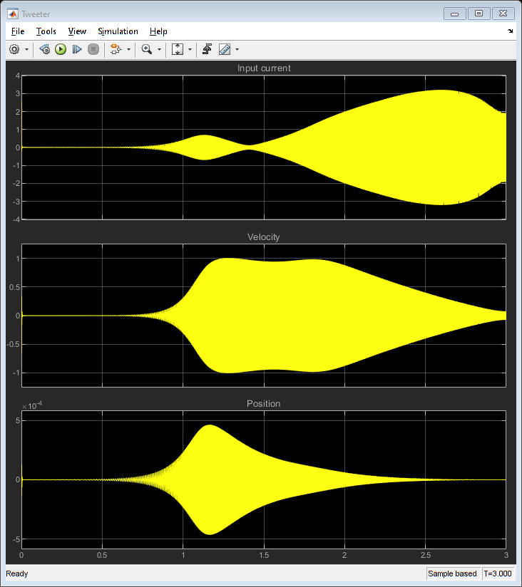
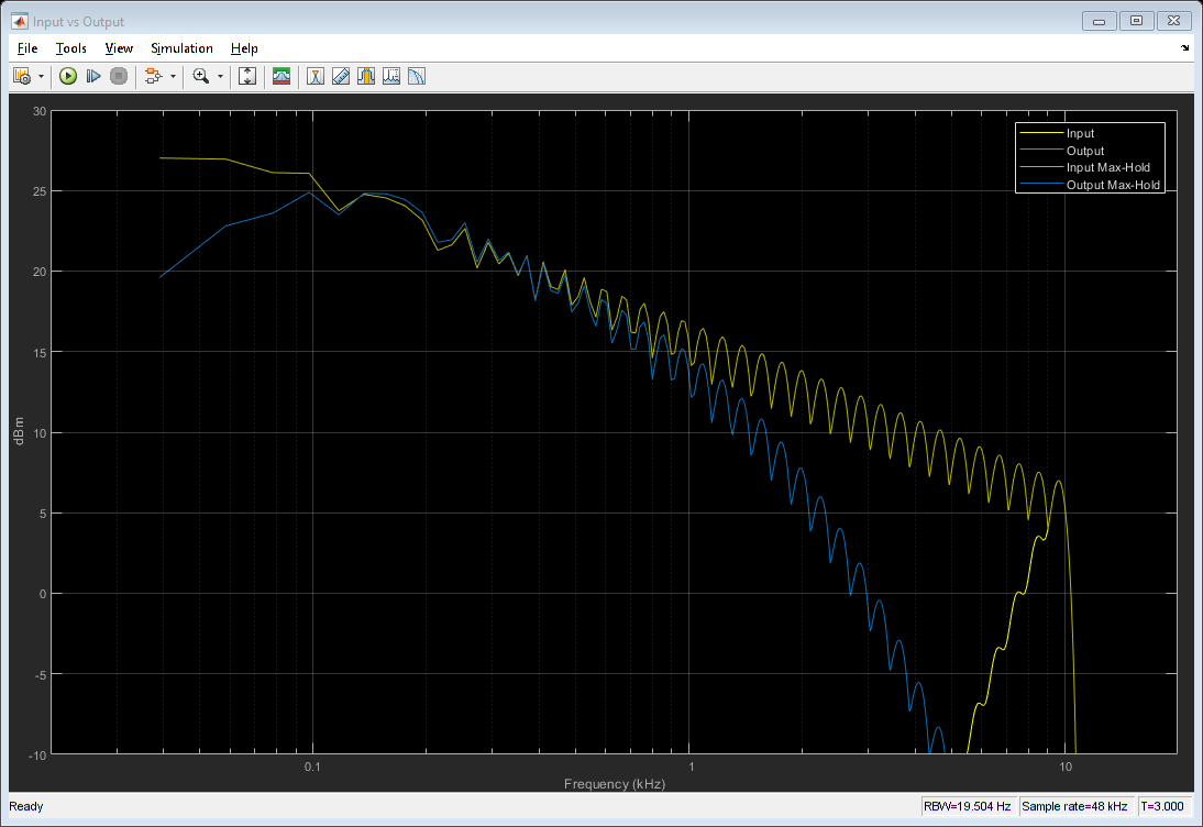
In addition to combining two physical domains in one simulation, digital signal processing algorithms can be included. The following model represents an active loudspeaker with a woofer and a tweeter. The crossover, parametric EQ and shelving filters are implemented in the digital domain, followed by an optimized power amplifier for each driver. The output of each driver is measured separately, and the combined output is compared to the log-chirp input in the frequency domain.
model = 'MixedModeling';
open_system(model);
sim(model,3);
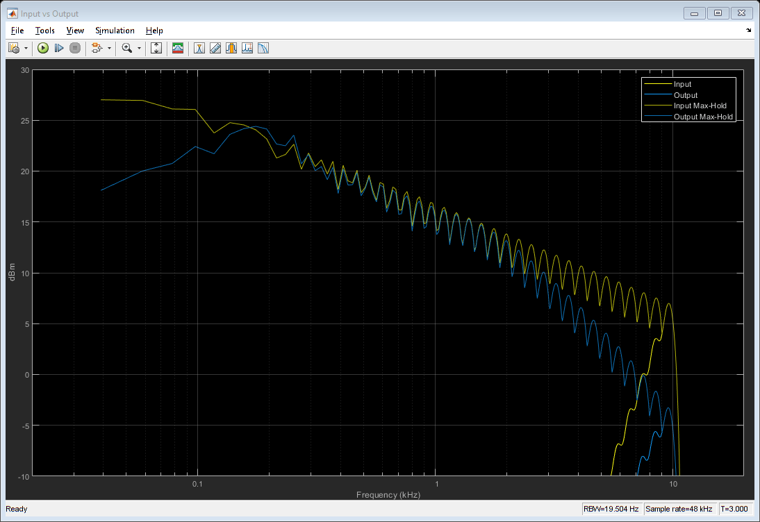
close_system(model,0)
Modeling Nonlinear Elements
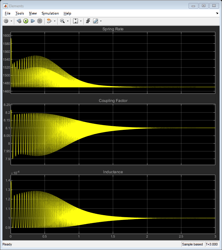
Several loudspeaker elements are nonlinear. For example, the voice coil force factor and inductance vary with its position in the magnet. Furthermore, the suspension spring rate changes at the extremities of its displacement range.
Linear components in the previous model can be replaced by custom versions that implement the nonlinearities that are required. For example, the spring component can define the spring rate  as
as  , where
  is the displacement and
  are the polynomial coefficients (
 being the spring rate at displacement zero).
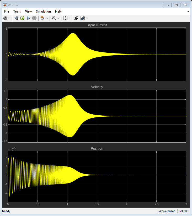
Plot sample values for compliance, force factor and inductance. Run model that implements the "woofer" driver of the previous model, but with three linear components replaced by nonlinear components.
plotNonLinearBHK;

model = 'NonLinearBHK';
open_system(model);
sim(model,3);
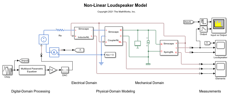

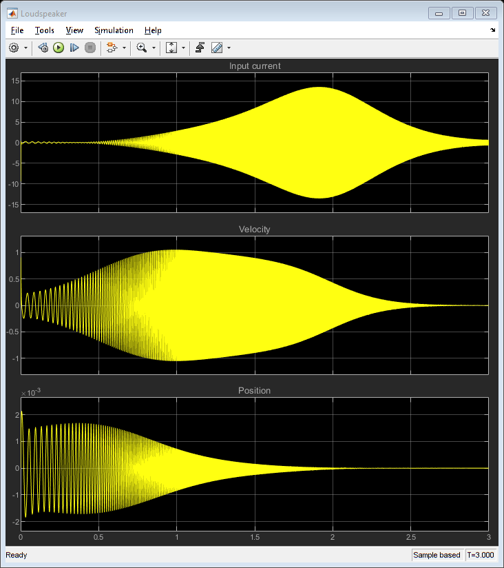
close_system(model,0)
Starting from these examples, add components to model an enclosure, or implement your own nonlinear elements. Simscape™ will allow you to do this using the domain of your choice (electrical, mechanical). You can also test any digital pre-processing that is required, all in one model.
Definitions
input voltage
input current
voice coil inductance
voice coil resistance
force factor
 force applied to the diaphragm
diaphragm velocity
 diaphragm displacement
moving mass
mechanical loss
suspension compliance
acoustical impedance