Exploring Genome-Wide Differences in DNA Methylation Profiles
This example shows how to perform a genome-wide analysis of DNA methylation in the human by using genome sequencing.
Note: For enhanced performance, MathWorks recommends that you run this example on a 64-bit platform, because the memory footprint is close to 2 GB. On a 32-bit platform, if you receive "Out of memory" errors when running this example, try increasing the virtual memory (or swap space) of your operating system or try setting the 3GB switch (32-bit Windows® XP only). For details, see Resolve “Out of Memory” Errors.
Introduction
DNA methylation is an epigenetic modification that modulates gene expression and the maintenance of genomic organization in normal and disease processes. DNA methylation can define different states of the cell, and it is inheritable during cell replication. Aberrant DNA methylation patterns have been associated with cancer and tumor suppressor genes.
In this example you will explore the DNA methylation profiles of two human cancer cells: parental HCT116 colon cancer cells and DICERex5 cells. DICERex5 cells are derived from HCT116 cells after the truncation of the DICER1 alleles. Serre et al. in [1] proposed to study DNA methylation profiles by using the MBD2 protein as a methyl CpG binding domain and subsequently used high-throughput sequencing (HTseq). This technique is commonly known as MBD-Seq. Short reads for two replicates of the two samples have been submitted to NCBI's SRA archive by the authors of [1]. There are other technologies available to interrogate DNA methylation status of CpG sites in combination with HTseq, for example MeDIP-seq or the use of restriction enzymes. You can also analyze this type of data sets following the approach presented in this example.
Data Sets
You can obtain the unmapped single-end reads for four sequencing experiments from NCBI. Short reads were produced using Illumina®'s Genome Analyzer II. Average insert size is 120 bp, and the length of short reads is 36 bp.
This example assumes that you:
(1) downloaded the files SRR030222.sra, SRR030223.sra, SRR030224.sra and SRR030225.sra containing the unmapped short reads for two replicates of from the DICERex5 sample and two replicates from the HCT116 sample respectively, from NCBI SRA Run Selector and converted them to FASTQ-formatted files using the NCBI SRA Toolkit.
(2) produced SAM-formatted files by mapping the short reads to the reference human genome (NCBI Build 37.5) using the Bowtie [2] algorithm. Only uniquely mapped reads are reported.
(3) compressed the SAM formatted files to BAM and ordered them by reference name first, then by genomic position by using SAMtools [3].
This example also assumes that you downloaded the reference human genome (GRCh37.p5). You can use the bowtie-inspect command to reconstruct the human reference directly from the bowtie indices. Or you may download the reference from the NCBI repository by uncommenting the following line:
% getgenbank('NC_000009','FileFormat','fasta','tofile','hsch9.fasta');
Creating a MATLAB® Interface to the BAM-Formatted Files
To explore the signal coverage of the HCT116 samples you need to construct a BioMap. BioMap has an interface that provides direct access to the mapped short reads stored in the BAM-formatted file, thus minimizing the amount of data that is actually loaded into memory. Use the function baminfo to obtain a list of the existing references and the actual number of short reads mapped to each one.
info = baminfo('SRR030224.bam','ScanDictionary',true);
fprintf('%-35s%s\n','Reference','Number of Reads');
for i = 1:numel(info.ScannedDictionary)
    fprintf('%-35s%d\n',info.ScannedDictionary{i},...
        info.ScannedDictionaryCount(i));
end
Reference                          Number of Reads
gi|224589800|ref|NC_000001.10|     205065
gi|224589811|ref|NC_000002.11|     187019
gi|224589815|ref|NC_000003.11|     73986
gi|224589816|ref|NC_000004.11|     84033
gi|224589817|ref|NC_000005.9|      96898
gi|224589818|ref|NC_000006.11|     87990
gi|224589819|ref|NC_000007.13|     120816
gi|224589820|ref|NC_000008.10|     111229
gi|224589821|ref|NC_000009.11|     106189
gi|224589801|ref|NC_000010.10|     112279
gi|224589802|ref|NC_000011.9|      104466
gi|224589803|ref|NC_000012.11|     87091
gi|224589804|ref|NC_000013.10|     53638
gi|224589805|ref|NC_000014.8|      64049
gi|224589806|ref|NC_000015.9|      60183
gi|224589807|ref|NC_000016.9|      146868
gi|224589808|ref|NC_000017.10|     195893
gi|224589809|ref|NC_000018.9|      60344
gi|224589810|ref|NC_000019.9|      166420
gi|224589812|ref|NC_000020.10|     148950
gi|224589813|ref|NC_000021.8|      310048
gi|224589814|ref|NC_000022.10|     76037
gi|224589822|ref|NC_000023.10|     32421
gi|224589823|ref|NC_000024.9|      18870
gi|17981852|ref|NC_001807.4|       1015
Unmapped                           6805842
In this example you will focus on the analysis of chromosome 9. Create a BioMap for the two HCT116 sample replicates.
bm_hct116_1 = BioMap('SRR030224.bam','SelectRef','gi|224589821|ref|NC_000009.11|')
bm_hct116_2 = BioMap('SRR030225.bam','SelectRef','gi|224589821|ref|NC_000009.11|')
bm_hct116_1 =

  BioMap with properties:

    SequenceDictionary: 'gi|224589821|ref|NC_000009.11|'
             Reference: [106189x1 File indexed property]
             Signature: [106189x1 File indexed property]
                 Start: [106189x1 File indexed property]
        MappingQuality: [106189x1 File indexed property]
                  Flag: [106189x1 File indexed property]
          MatePosition: [106189x1 File indexed property]
               Quality: [106189x1 File indexed property]
              Sequence: [106189x1 File indexed property]
                Header: [106189x1 File indexed property]
                 NSeqs: 106189
                  Name: ''


bm_hct116_2 =

  BioMap with properties:

    SequenceDictionary: 'gi|224589821|ref|NC_000009.11|'
             Reference: [107586x1 File indexed property]
             Signature: [107586x1 File indexed property]
                 Start: [107586x1 File indexed property]
        MappingQuality: [107586x1 File indexed property]
                  Flag: [107586x1 File indexed property]
          MatePosition: [107586x1 File indexed property]
               Quality: [107586x1 File indexed property]
              Sequence: [107586x1 File indexed property]
                Header: [107586x1 File indexed property]
                 NSeqs: 107586
                  Name: ''
Using a binning algorithm provided by the getBaseCoverage method, you can plot the coverage of both replicates for an initial inspection. For reference, you can also add the ideogram for the human chromosome 9 to the plot using the chromosomeplot function.
figure
ha = gca;
hold on
n = 141213431;               % length of chromosome 9
[cov,bin] = getBaseCoverage(bm_hct116_1,1,n,'binWidth',100);
h1 = plot(bin,cov,'b');      % plots the binned coverage of bm_hct116_1
[cov,bin] = getBaseCoverage(bm_hct116_2,1,n,'binWidth',100);
h2 = plot(bin,cov,'g');      % plots the binned coverage of bm_hct116_2
chromosomeplot('hs_cytoBand.txt', 9, 'AddToPlot', ha) % plots an ideogram along the x-axis
axis(ha,[1 n 0 100])         % zooms-in the y-axis
fixGenomicPositionLabels(ha) % formats tick labels and adds datacursors
legend([h1 h2],'HCT116-1','HCT116-2','Location','NorthEast')
ylabel('Coverage')
title('Coverage for two replicates of the HCT116 sample')
fig = gcf;
fig.Position = max(fig.Position,[0 0 900 0]); % resize window
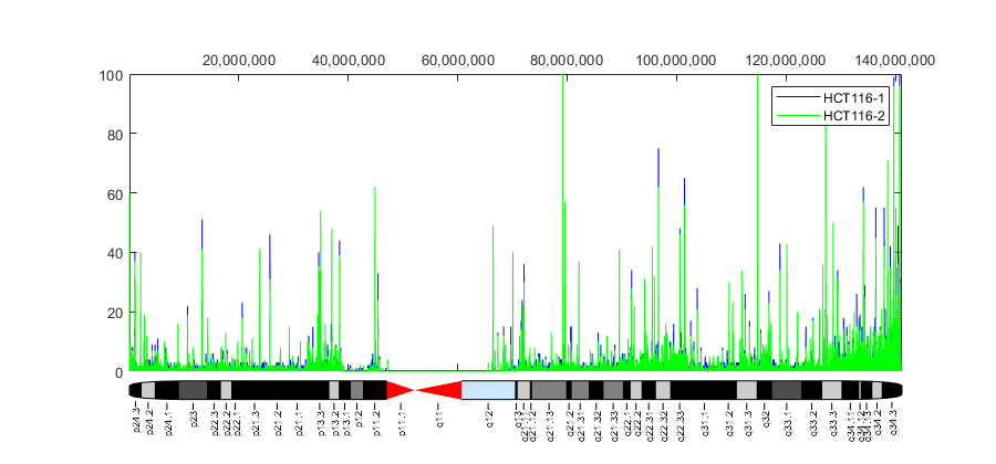
Because short reads represent the methylated regions of the DNA, there is a correlation between aligned coverage and DNA methylation. Observe the increased DNA methylation close to the chromosome telomeres; it is known that there is an association between DNA methylation and the role of telomeres for maintaining the integrity of the chromosomes. In the coverage plot you can also see a long gap over the chromosome centromere. This is due to the repetitive sequences present in the centromere, which prevent us from aligning short reads to a unique position in this region. In the data sets used in this example only about 30% of the short reads were uniquely mapped to the reference genome.
Correlating CpG Islands and DNA Methylation
DNA methylation normally occurs in CpG dinucleotides. Alteration of the DNA methylation patterns can lead to transcriptional silencing, especially in the gene promoter CpG islands. But, it is also known that DNA methylation can block CTCF binding and can silence miRNA transcription among other relevant functions. In general, it is expected that mapped reads should preferably align to CpG rich regions.
Load the human chromosome 9 from the reference file hs37.fasta. For this example, it is assumed that you recovered the reference from the Bowtie indices using the bowtie-inspect command; therefore hs37.fasta contains all the human chromosomes. To load only the chromosome 9 you can use the option nave-value pair BLOCKREAD with the fastaread function.
chr9 = fastaread('hs37.fasta','blockread',9);
chr9.Header
ans =

    'gi|224589821|ref|NC_000009.11| Homo sapiens chromosome 9, GRCh37 primary reference assembly'
Use the cpgisland function to find the CpG clusters. Using the standard definition for CpG islands [4], 200 or more bp islands with 60% or greater CpGobserved/CpGexpected ratio, leads to 1682 GpG islands found in chromosome 9.
cpgi = cpgisland(chr9.Sequence)
cpgi =

  struct with fields:

    Starts: [10783 29188 73049 73686 113309 114488 116877 … ] (1×1682 double)
     Stops: [11319 29409 73624 73893 114336 114809 117105 … ] (1×1682 double)
Use the getCounts method to calculate the ratio of aligned bases that are inside CpG islands. For the first replicate of the sample HCT116, the ratio is close to 45%.
aligned_bases_in_CpG_islands = getCounts(bm_hct116_1,cpgi.Starts,cpgi.Stops,'method','sum')
aligned_bases_total = getCounts(bm_hct116_1,1,n,'method','sum')
ratio = aligned_bases_in_CpG_islands ./ aligned_bases_total
aligned_bases_in_CpG_islands =

     1724363


aligned_bases_total =

     3822804


ratio =

    0.4511
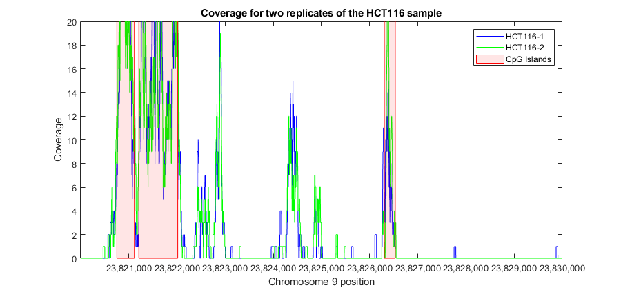
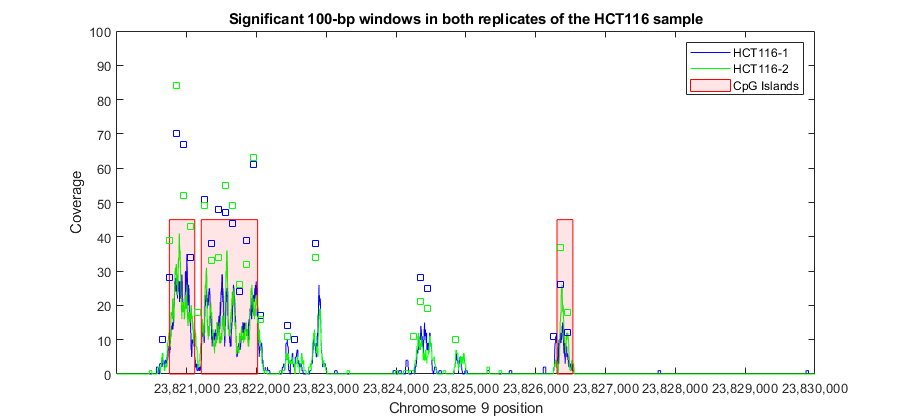
You can explore high resolution coverage plots of the two sample replicates and observe how the signal correlates with the CpG islands. For example, explore the region between 23,820,000 and 23,830,000 bp. This is the 5' region of the human gene ELAVL2.
r1 = 23820001; % set the region limits
r2 = 23830000;
fhELAVL2 = figure; % keep the figure handle to use it later
hold on
% plot high-resolution coverage of bm_hct116_1
h1 = plot(r1:r2,getBaseCoverage(bm_hct116_1,r1,r2,'binWidth',1),'b');
% plot high-resolution coverage of bm_hct116_2
h2 = plot(r1:r2,getBaseCoverage(bm_hct116_2,r1,r2,'binWidth',1),'g');

% mark the CpG islands within the [r1 r2] region
for i = 1:numel(cpgi.Starts)
    if cpgi.Starts(i)>r1 && cpgi.Stops(i)<r2 % is CpG island inside [r1 r2]?
        px = [cpgi.Starts([i i]) cpgi.Stops([i i])]; % x-coordinates for patch
        py = [0 max(ylim) max(ylim) 0];              % y-coordinates for patch
        hp = patch(px,py,'r','FaceAlpha',.1,'EdgeColor','r','Tag','cpgi');
    end
end

axis([r1 r2 0 20])            % zooms-in the y-axis
fixGenomicPositionLabels(gca) % formats tick labels and adds datacursors
legend([h1 h2 hp],'HCT116-1','HCT116-2','CpG Islands')
ylabel('Coverage')
xlabel('Chromosome 9 position')
title('Coverage for two replicates of the HCT116 sample')
Statistical Modelling of Count Data
To find regions that contain more mapped reads than would be expected by chance, you can follow a similar approach to the one described by Serre et al. [1]. The number of counts for non-overlapping contiguous 100 bp windows is statistically modeled.
First, use the getCounts method to count the number of mapped reads that start at each window. In this example you use a binning approach that considers only the start position of every mapped read, following the approach of Serre et al. However, you may also use the OVERLAP and METHOD name-value pairs in getCounts to compute more accurate statistics. For instance, to obtain the maximum coverage for each window considering base pair resolution, set OVERLAP to 1 and METHOD to MAX.
n = numel(chr9.Sequence); % length of chromosome
w = 1:100:n; % windows of 100 bp

counts_1 = getCounts(bm_hct116_1,w,w+99,'independent',true,'overlap','start');
counts_2 = getCounts(bm_hct116_2,w,w+99,'independent',true,'overlap','start');
First, try to model the counts assuming that all the windows with counts are biologically significant and therefore from the same distribution. Use the negative bionomial distribution to fit a model the count data.
nbp = nbinfit(counts_1);
Plot the fitted model over a histogram of the empirical data.
figure
hold on
edges = 0:100;
emphist = histcounts(counts_1,edges); % calculate the empirical distribution
binCenters = (edges(1:end-1) + edges(2:end)) / 2;
bar(binCenters,emphist./sum(emphist),'c','grouped') % plot histogram
plot(0:100,nbinpdf(0:100,nbp(1),nbp(2)),'b','linewidth',2); % plot fitted model
axis([0 50 0 .001])
legend('Empirical Distribution','Negative Binomial Fit')
ylabel('Frequency')
xlabel('Counts')
title('Frequency of counts, 100bp windows (HCT116-1)')
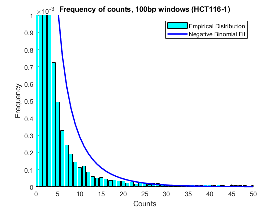
The poor fitting indicates that the observed distribution may be due to the mixture of two models, one that represents the background and one that represents the count data in methylated DNA windows.
A more realistic scenario would be to assume that windows with a small number of mapped reads are mainly the background (or null model). Serre et al. assumed that 100-bp windows containing four or more reads are unlikely to be generated by chance. To estimate a good approximation to the null model, you can fit the left body of the empirical distribution to a truncated negative binomial distribution. To fit a truncated distribution use the mle function. First you need to define an anonymous function that defines the right-truncated version of nbinpdf.
rtnbinpdf = @(x,p1,p2,t) nbinpdf(x,p1,p2) ./ nbincdf(t-1,p1,p2);
Define the fitting function using another anonymous function.
rtnbinfit = @(x2,t) mle(x2,'pdf',@(x3,p1,p2) rtnbinpdf(x3,p1,p2,t),'start',nbinfit(x2),'lower',[0 0]);
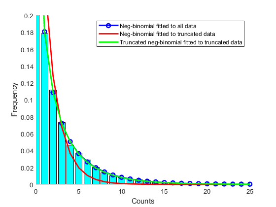
Before fitting the real data, let us assess the fitting procedure with some sampled data from a known distribution.
nbp = [0.5 0.2];              % Known coefficients
x = nbinrnd(nbp(1),nbp(2),10000,1); % Random sample
trun = 6;                     % Set a truncation threshold

nbphat1 = nbinfit(x);         % Fit non-truncated model to all data
nbphat2 = nbinfit(x(x<trun)); % Fit non-truncated model to truncated data (wrong)
nbphat3 = rtnbinfit(x(x<trun),trun); % Fit truncated model to truncated data

figure
hold on
edges = 0:100;
emphist = histcounts(x,edges);     % Calculate the empirical distribution
binCenters = (edges(1:end-1) + edges(2:end)) / 2;
bar(binCenters,emphist./sum(emphist),'c','grouped') % plot histogram
h1 = plot(0:100,nbinpdf(0:100,nbphat1(1),nbphat1(2)),'b-o','linewidth',2);
h2 = plot(0:100,nbinpdf(0:100,nbphat2(1),nbphat2(2)),'r','linewidth',2);
h3 = plot(0:100,nbinpdf(0:100,nbphat3(1),nbphat3(2)),'g','linewidth',2);
axis([0 25 0 .2])
legend([h1 h2 h3],'Neg-binomial fitted to all data',...
    'Neg-binomial fitted to truncated data',...
    'Truncated neg-binomial fitted to truncated data')
ylabel('Frequency')
xlabel('Counts')
Identifying Significant Methylated Regions
For the two replicates of the HCT116 sample, fit a right-truncated negative binomial distribution to the observed null model using the rtnbinfit anonymous function previously defined.
trun = 4;  % Set a truncation threshold (as in [1])
pn1 = rtnbinfit(counts_1(counts_1<trun),trun); % Fit to HCT116-1 counts
pn2 = rtnbinfit(counts_2(counts_2<trun),trun); % Fit to HCT116-2 counts
Calculate the p-value for each window to the null distribution.
pval1 = 1 - nbincdf(counts_1,pn1(1),pn1(2));
pval2 = 1 - nbincdf(counts_2,pn2(1),pn2(2));
Calculate the false discovery rate using the mafdr function. Use the name-value pair BHFDR to use the linear-step up (LSU) procedure ([6]) to calculate the FDR adjusted p-values. Setting the FDR < 0.01 permits you to identify the 100-bp windows that are significantly methylated.
fdr1 = mafdr(pval1,'bhfdr',true);
fdr2 = mafdr(pval2,'bhfdr',true);

w1 = fdr1<.01; % logical vector indicating significant windows in HCT116-1
w2 = fdr2<.01; % logical vector indicating significant windows in HCT116-2
w12 = w1 & w2; % logical vector indicating significant windows in both replicates

Number_of_sig_windows_HCT116_1 = sum(w1)
Number_of_sig_windows_HCT116_2 = sum(w2)
Number_of_sig_windows_HCT116 = sum(w12)
Number_of_sig_windows_HCT116_1 =

        1662


Number_of_sig_windows_HCT116_2 =

        1674


Number_of_sig_windows_HCT116 =

        1346
Overall, you identified 1662 and 1674 non-overlapping 100-bp windows in the two replicates of the HCT116 samples, which indicates there is significant evidence of DNA methylation. There are 1346 windows that are significant in both replicates.
For example, looking again in the promoter region of the ELAVL2 human gene you can observe that in both sample replicates, multiple 100-bp windows have been marked significant.
figure(fhELAVL2) % bring back to focus the previously plotted figure
plot(w(w1)+50,counts_1(w1),'bs', 'HandleVisibility','off') % plot significant windows in HCT116-1
plot(w(w2)+50,counts_2(w2),'gs', 'HandleVisibility','off') % plot significant windows in HCT116-2
axis([r1 r2 0 100])
title('Significant 100-bp windows in both replicates of the HCT116 sample')
Finding Genes With Significant Methylated Promoter Regions
DNA methylation is involved in the modulation of gene expression. For instance, it is well known that hypermethylation is associated with the inactivation of several tumor suppressor genes. You can study in this data set the methylation of gene promoter regions.
First, download from Ensembl a tab-separated-value (TSV) table with all protein encoding genes to a text file, ensemblmart_genes_hum37.txt. For this example, we are using Ensembl release 64. Using Ensembl's BioMart service, you can select a table with the following attributes: chromosome name, gene biotype, gene name, gene start/end, and strand direction.
Use the provided helper function ensemblmart2gff to convert the downloaded TSV file to a GFF formatted file. Then use GFFAnnotation to load the file into MATLAB and create a subset with the genes present in chromosome 9 only. This results 800 annotated protein-coding genes in the Ensembl database.
GFFfilename = ensemblmart2gff('ensemblmart_genes_hum37.txt');
a = GFFAnnotation(GFFfilename)
a9 = getSubset(a,'reference','9')
numGenes = a9.NumEntries
a =

  GFFAnnotation with properties:

    FieldNames: {1×9 cell}
    NumEntries: 21184


a9 =

  GFFAnnotation with properties:

    FieldNames: {1×9 cell}
    NumEntries: 800


numGenes =

   800
Find the promoter regions for each gene. In this example we consider the proximal promoter as the -500/100 upstream region.
downstream = 500;
upstream   = 100;

geneDir = strcmp(a9.Strand,'+');  % logical vector indicating strands in the forward direction

% calculate promoter's start position for genes in the forward direction
promoterStart(geneDir) = a9.Start(geneDir) - downstream;
% calculate promoter's end position for genes in the forward direction
promoterStop(geneDir) = a9.Start(geneDir) + upstream;
% calculate promoter's start position for genes in the reverse direction
promoterStart(~geneDir) = a9.Stop(~geneDir) - upstream;
% calculate promoter's end position for genes in the reverse direction
promoterStop(~geneDir) = a9.Stop(~geneDir) + downstream;
Use a dataset as a container for the promoter information, as we can later add new columns to store gene counts and p-values.
promoters = dataset({a9.Feature,'Gene'});
promoters.Strand = char(a9.Strand);
promoters.Start = promoterStart';
promoters.Stop = promoterStop';
Find genes with significant DNA methylation in the promoter region by looking at the number of mapped short reads that overlap at least one base pair in the defined promoter region.
promoters.Counts_1 = getCounts(bm_hct116_1,promoters.Start,promoters.Stop,...
    'overlap',1,'independent',true);
promoters.Counts_2 = getCounts(bm_hct116_2,promoters.Start,promoters.Stop,...
    'overlap',1,'independent',true);
Fit a null distribution for each sample replicate and compute the p-values:
trun = 5;  % Set a truncation threshold
pn1 = rtnbinfit(promoters.Counts_1(promoters.Counts_1<trun),trun); % Fit to HCT116-1 promoter counts
pn2 = rtnbinfit(promoters.Counts_2(promoters.Counts_2<trun),trun); % Fit to HCT116-2 promoter counts
promoters.pval_1 = 1 - nbincdf(promoters.Counts_1,pn1(1),pn1(2)); % p-value for every promoter in HCT116-1
promoters.pval_2 = 1 - nbincdf(promoters.Counts_2,pn2(1),pn2(2)); % p-value for every promoter in HCT116-2

Number_of_sig_promoters =  sum(promoters.pval_1<.01 & promoters.pval_2<.01)

Ratio_of_sig_methylated_promoters = Number_of_sig_promoters./numGenes
Number_of_sig_promoters =

    74


Ratio_of_sig_methylated_promoters =

    0.0925
Observe that only 74 (out of 800) genes in chromosome 9 have significantly DNA methylated regions (pval<0.01 in both replicates). Display a report of the 30 genes with the most significant methylated promoter regions.
[~,order] = sort(promoters.pval_1.*promoters.pval_2);
promoters(order(1:30),[1 2 3 4 5 7 6 8])
ans =

    Gene                   Strand    Start        Stop         Counts_1
    {'DMRT3'      }        +            976464       977064    223
    {'CNTFR'      }        -          34590021     34590621    219
    {'GABBR2'     }        -         101471379    101471979    404
    {'CACNA1B'    }        +         140771741    140772341    454
    {'BARX1'      }        -          96717554     96718154    264
    {'FAM78A'     }        -         134151834    134152434    497
    {'FOXB2'      }        +          79634071     79634671    163
    {'TLE4'       }        +          82186188     82186788    157
    {'ASTN2'      }        -         120177248    120177848    141
    {'FOXE1'      }        +         100615036    100615636    149
    {'MPDZ'       }        -          13279489     13280089    129
    {'PTPRD'      }        -          10612623     10613223    145
    {'PALM2-AKAP2'}        +         112542089    112542689    134
    {'FAM69B'     }        +         139606522    139607122    112
    {'WNK2'       }        +          95946698     95947298    108
    {'IGFBPL1'    }        -          38424344     38424944    110
    {'AKAP2'      }        +         112542269    112542869    107
    {'C9orf4'     }        -         111929471    111930071    102
    {'COL5A1'     }        +         137533120    137533720     84
    {'LHX3'       }        -         139096855    139097455     74
    {'OLFM1'      }        +         137966768    137967368     75
    {'NPR2'       }        +          35791651     35792251     68
    {'DBC1'       }        -         122131645    122132245     61
    {'SOHLH1'     }        -         138591274    138591874     56
    {'PIP5K1B'    }        +          71320075     71320675     59
    {'PRDM12'     }        +         133539481    133540081     53
    {'ELAVL2'     }        -          23826235     23826835     50
    {'ZFP37'      }        -         115818939    115819539     59
    {'RP11-35N6.1'}        +         103790491    103791091     60
    {'DMRT2'      }        +           1049854      1050454     54


    pval_1        Counts_2    pval_2
    6.6613e-16    253         5.5511e-16
    6.6613e-16    226         5.5511e-16
    6.6613e-16    400         5.5511e-16
    6.6613e-16    408         5.5511e-16
    6.6613e-16    286         5.5511e-16
    6.6613e-16    499         5.5511e-16
       1.4e-13    165         6.0352e-13
    3.5649e-13    151         4.7347e-12
    4.3566e-12    163         8.0969e-13
    1.2447e-12    133         6.7598e-11
    2.8679e-11    148         7.3682e-12
    2.3279e-12    127         1.6448e-10
    1.3068e-11    135         5.0276e-11
    4.1911e-10    144         1.3295e-11
     7.897e-10    125         2.2131e-10
    5.7523e-10    114         1.1364e-09
    9.2538e-10    106         3.7513e-09
    2.0467e-09     96         1.6795e-08
    3.6266e-08     97         1.4452e-08
    1.8171e-07     91         3.5644e-08
    1.5457e-07     69         1.0074e-06
    4.8093e-07     73         5.4629e-07
    1.5082e-06     62         2.9575e-06
    3.4322e-06     67         1.3692e-06
    2.0943e-06     63         2.5345e-06
    5.6364e-06     61         3.4518e-06
    9.2778e-06     62         2.9575e-06
    2.0943e-06     47         3.0746e-05
    1.7771e-06     42         6.8037e-05
    4.7762e-06     46         3.6016e-05
Finding Intergenic Regions that are Significantly Methylated
Serre et al. [1] reported that, in these data sets, approximately 90% of the uniquely mapped reads fall outside the 5' gene promoter regions. Using a similar approach as before, you can find genes that have intergenic methylated regions. To compensate for the varying lengths of the genes, you can use the maximum coverage, computed base-by-base, instead of the raw number of mapped short reads. Another alternative approach to normalize the counts by the gene length is to set the METHOD name-value pair to rpkm in the getCounts function.
intergenic = dataset({a9.Feature,'Gene'});
intergenic.Strand = char(a9.Strand);
intergenic.Start = a9.Start;
intergenic.Stop = a9.Stop;

intergenic.Counts_1 = getCounts(bm_hct116_1,intergenic.Start,intergenic.Stop,...
    'overlap','full','method','max','independent',true);
intergenic.Counts_2 = getCounts(bm_hct116_2,intergenic.Start,intergenic.Stop,...
    'overlap','full','method','max','independent',true);
trun = 10; % Set a truncation threshold
pn1 = rtnbinfit(intergenic.Counts_1(intergenic.Counts_1<trun),trun); % Fit to HCT116-1 intergenic counts
pn2 = rtnbinfit(intergenic.Counts_2(intergenic.Counts_2<trun),trun); % Fit to HCT116-2 intergenic counts
intergenic.pval_1 = 1 - nbincdf(intergenic.Counts_1,pn1(1),pn1(2)); % p-value for every intergenic region in HCT116-1
intergenic.pval_2 = 1 - nbincdf(intergenic.Counts_2,pn2(1),pn2(2)); % p-value for every intergenic region in HCT116-2

Number_of_sig_genes =  sum(intergenic.pval_1<.01 & intergenic.pval_2<.01)

Ratio_of_sig_methylated_genes = Number_of_sig_genes./numGenes

[~,order] = sort(intergenic.pval_1.*intergenic.pval_2);

intergenic(order(1:30),[1 2 3 4 5 7 6 8])
Number_of_sig_genes =

    62


Ratio_of_sig_methylated_genes =

    0.0775


ans =

    Gene                  Strand    Start        Stop         Counts_1
    {'AL772363.1'}        -         140762377    140787022    106
    {'CACNA1B'   }        +         140772241    141019076    106
    {'SUSD1'     }        -         114803065    114937688     88
    {'C9orf172'  }        +         139738867    139741797     99
    {'NR5A1'     }        -         127243516    127269709     86
    {'BARX1'     }        -          96713628     96717654     77
    {'KCNT1'     }        +         138594031    138684992     58
    {'GABBR2'    }        -         101050391    101471479     65
    {'FOXB2'     }        +          79634571     79635869     51
    {'NDOR1'     }        +         140100119    140113813     54
    {'KIAA1045'  }        +          34957484     34984679     50
    {'ADAMTSL2'  }        +         136397286    136440641     55
    {'PAX5'      }        -          36833272     37034476     48
    {'OLFM1'     }        +         137967268    138013025     55
    {'PBX3'      }        +         128508551    128729656     45
    {'FOXE1'     }        +         100615536    100618986     49
    {'MPDZ'      }        -          13105703     13279589     51
    {'ASTN2'     }        -         119187504    120177348     43
    {'ARRDC1'    }        +         140500106    140509812     49
    {'IGFBPL1'   }        -          38408991     38424444     45
    {'LHX3'      }        -         139088096    139096955     44
    {'PAPPA'     }        +         118916083    119164601     44
    {'CNTFR'     }        -          34551430     34590121     41
    {'DMRT3'     }        +            976964       991731     40
    {'TUSC1'     }        -          25676396     25678856     46
    {'ELAVL2'    }        -          23690102     23826335     35
    {'SMARCA2'   }        +           2015342      2193624     36
    {'GAS1'      }        -          89559279     89562104     34
    {'GRIN1'     }        +         140032842    140063207     36
    {'TLE4'      }        +          82186688     82341658     36


    pval_1        Counts_2    pval_2
    8.6597e-15     98         1.8763e-14
    8.6597e-15     98         1.8763e-14
    2.2904e-12    112         7.7716e-16
    7.4718e-14     96         3.5749e-14
     4.268e-12     90         2.5457e-13
    7.0112e-11     62          2.569e-09
    2.5424e-08     73         6.9019e-11
    2.9078e-09     58         9.5469e-09
    2.2131e-07     58         9.5469e-09
    8.7601e-08     55         2.5525e-08
    3.0134e-07     55         2.5525e-08
    6.4307e-08     45         6.7163e-07
     5.585e-07     49         1.8188e-07
    6.4307e-08     42         1.7861e-06
    1.4079e-06     51         9.4566e-08
    4.1027e-07     46         4.8461e-07
    2.2131e-07     42         1.7861e-06
    2.6058e-06     43         1.2894e-06
    4.1027e-07     36         1.2564e-05
    1.4079e-06     39         4.7417e-06
    1.9155e-06     36         1.2564e-05
    1.9155e-06     35         1.7377e-05
    4.8199e-06     37         9.0815e-06
    6.5537e-06     37         9.0815e-06
    1.0346e-06     31         6.3417e-05
    3.0371e-05     41         2.4736e-06
    2.2358e-05     40         3.4251e-06
    4.1245e-05     41         2.4736e-06
    2.2358e-05     38         6.5629e-06
    2.2358e-05     37         9.0815e-06
For instance, explore the methylation profile of the BARX1 gene, the sixth significant gene with intergenic methylation in the previous list. The GTF formatted file ensemblmart_barx1.gtf contains structural information for this gene obtained from Ensembl using the BioMart service.
Use GTFAnnotation to load the structural information into MATLAB. There are two annotated transcripts for this gene.
barx1 = GTFAnnotation('ensemblmart_barx1.gtf')
transcripts = getTranscriptNames(barx1)
barx1 =

  GTFAnnotation with properties:

    FieldNames: {1×11 cell}
    NumEntries: 18


transcripts =

  2×1 cell array

    {'ENST00000253968'}
    {'ENST00000401724'}
Plot the DNA methylation profile for both HCT116 sample replicates with base-pair resolution. Overlay the CpG islands and plot the exons for each of the two transcripts along the bottom of the plot.
range = barx1.getRange;
r1 = range(1)-1000; % set the region limits
r2 = range(2)+1000;
figure
hold on
% plot high-resolution coverage of bm_hct116_1
h1 = plot(r1:r2,getBaseCoverage(bm_hct116_1,r1,r2,'binWidth',1),'b');
% plot high-resolution coverage of bm_hct116_2
h2 = plot(r1:r2,getBaseCoverage(bm_hct116_2,r1,r2,'binWidth',1),'g');

% mark the CpG islands within the [r1 r2] region
for i = 1:numel(cpgi.Starts)
    if cpgi.Starts(i)>r1 && cpgi.Stops(i)<r2 % is CpG island inside [r1 r2]?
        px = [cpgi.Starts([i i]) cpgi.Stops([i i])];  % x-coordinates for patch
        py = [0 max(ylim) max(ylim) 0];               % y-coordinates for patch
        hp = patch(px,py,'r','FaceAlpha',.1,'EdgeColor','r','Tag','cpgi');
    end
end

% mark the exons at the bottom of the axes
for i = 1:numel(transcripts)
    exons = getSubset(barx1,'Transcript',transcripts{i},'Feature','exon');
    for j = 1:exons.NumEntries
        px = [exons.Start([j j]);exons.Stop([j j])]'; % x-coordinates for patch
        py = [0 1 1 0]-i*2-1;                         % y-coordinates for patch
        hq = patch(px,py,'b','FaceAlpha',.1,'EdgeColor','b','Tag','exon');
    end
end

axis([r1 r2 -numel(transcripts)*2-2 80])  % zooms-in the y-axis
fixGenomicPositionLabels(gca) % formats tick labels and adds datacursors
ylabel('Coverage')
xlabel('Chromosome 9 position')
title('High resolution coverage in the BARX1 gene')
legend([h1 h2 hp hq],'HCT116-1','HCT116-2','CpG Islands','Exons','Location','NorthWest')

Observe the highly methylated region in the 5' promoter region (right-most CpG island). Recall that for this gene transcription occurs in the reverse strand. More interesting, observe the highly methylated regions that overlap the initiation of each of the two annotated transcripts (two middle CpG islands).
Differential Analysis of Methylation Patterns
In the study by Serre et al. another cell line is also analyzed. New cells (DICERex5) are derived from the same HCT116 colon cancer cells after truncating the DICER1 alleles. It has been reported in literature [5] that there is a localized change of DNA methylation at small number of gene promoters. In this example, you will find significant 100-bp windows in two sample replicates of the DICERex5 cells following the same approach as the parental HCT116 cells, and then you will search statistically significant differences between the two cell lines.
The helper function getWindowCounts captures the similar steps to find windows with significant coverage as before. getWindowCounts returns vectors with counts, p-values, and false discovery rates for each new replicate.
bm_dicer_1 = BioMap('SRR030222.bam','SelectRef','gi|224589821|ref|NC_000009.11|');
bm_dicer_2 = BioMap('SRR030223.bam','SelectRef','gi|224589821|ref|NC_000009.11|');
[counts_3,pval3,fdr3] = getWindowCounts(bm_dicer_1,4,w,100);
[counts_4,pval4,fdr4] = getWindowCounts(bm_dicer_2,4,w,100);
w3 = fdr3<.01; % logical vector indicating significant windows in DICERex5_1
w4 = fdr4<.01; % logical vector indicating significant windows in DICERex5-2
w34 = w3 & w4; % logical vector indicating significant windows in both replicates
Number_of_sig_windows_DICERex5_1 = sum(w3)
Number_of_sig_windows_DICERex5_2 = sum(w4)
Number_of_sig_windows_DICERex5 = sum(w34)
Number_of_sig_windows_DICERex5_1 =

   908


Number_of_sig_windows_DICERex5_2 =

        1041


Number_of_sig_windows_DICERex5 =

   759
To perform a differential analysis you use the 100-bp windows that are significant in at least one of the samples (either HCT116 or DICERex5).
wd = w34 | w12; % logical vector indicating windows included in the diff. analysis

counts = [counts_1(wd) counts_2(wd) counts_3(wd) counts_4(wd)];
ws = w(wd); % window start for each row in counts
Use the function manorm to normalize the data. The PERCENTILE name-value pair lets you filter out windows with very large number of counts while normalizing, since these windows are mainly due to artifacts, such as repetitive regions in the reference chromosome.
counts_norm = round(manorm(counts,'percentile',90).*100);
Use the function mattest to perform a two-sample t-test to identify differentially covered windows from the two different cell lines.
pval = mattest(counts_norm(:,[1 2]),counts_norm(:,[3 4]),'bootstrap',true,...
    'showhist',true,'showplot',true);
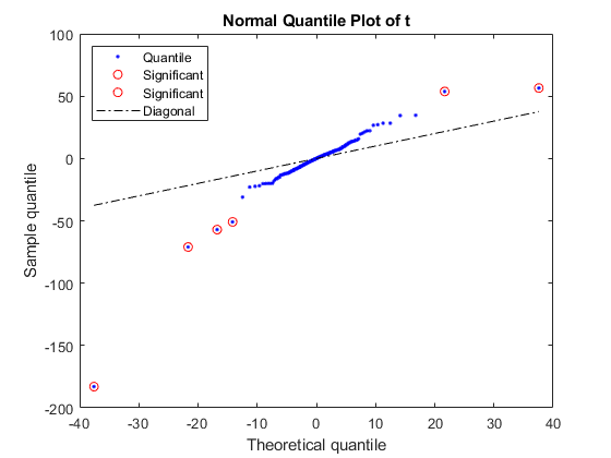
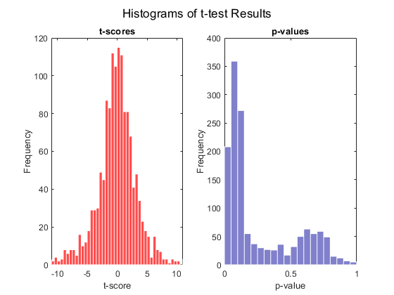
Create a report with the 25 most significant differentially covered windows. While creating the report use the helper function findClosestGene to determine if the window is intergenic, intragenic, or if it is in a proximal promoter region.
[~,ord] = sort(pval);
fprintf('Window Pos       Type                  p-value   HCT116     DICERex5\n\n');
for i = 1:25
    j = ord(i);
    [~,msg] = findClosestGene(a9,[ws(j) ws(j)+99]);
    fprintf('%10d  %-25s %7.6f%5d%5d %5d%5d\n',  ...
        ws(j),msg,pval(j),counts_norm(j,:));
end
Window Pos       Type                  p-value   HCT116     DICERex5

 140311701  Intergenic (EXD3)         0.000020   13   13   104  105
 139546501  Intragenic                0.001525   21   21    91   93
     10901  Intragenic                0.002222  258  257   434  428
 120176801  Intergenic (ASTN2)        0.002270  266  270   155  155
 139914801  Intergenic (ABCA2)        0.002482   64   63    26   25
 126128501  Intergenic (CRB2)         0.002664   94   93   129  130
  71939501  Prox. Promoter (FAM189A2) 0.004687  107  101     0    0
 124461001  Intergenic (DAB2IP)       0.004747   77   76    39   37
 140086501  Intergenic (TPRN)         0.005489   47   42   123  124
  79637201  Intragenic                0.006323   52   51    32   31
 136470801  Intragenic                0.006323   52   51    32   31
 140918001  Intergenic (CACNA1B)      0.006786  176  169    71   68
 100615901  Intergenic (FOXE1)        0.006969  262  253   123  118
  98221901  Intergenic (PTCH1)        0.008291   26   30   104   99
 138730601  Intergenic (CAMSAP1)      0.008602   26   21    97   93
  89561701  Intergenic (GAS1)         0.008653   77   76     6   12
    977401  Intergenic (DMRT3)        0.008678  236  245   129  124
  37002601  Intergenic (PAX5)         0.008822  133  127   207  211
 139744401  Intergenic (PHPT1)        0.009078   47   46    32   31
 126771301  Intragenic                0.009547   43   46    97   93
  93922501  Intragenic                0.009565   34   34   149  161
  94187101  Intragenic                0.009579   73   80     6    6
 136044401  Intragenic                0.009623   39   34   110  105
 139611201  Intergenic (FAM69B)       0.009623   39   34   110  105
 139716201  Intergenic (C9orf86)      0.009860   73   72   136  130
Plot the DNA methylation profile for the promoter region of gene FAM189A2, the most significant differentially covered promoter region from the previous list. Overlay the CpG islands and the FAM189A2 gene.
range = getRange(getSubset(a9,'Feature','FAM189A2'));
r1 = range(1)-1000;
r2 = range(2)+1000;
figure
hold on

% plot high-resolution coverage of all replicates
h1 = plot(r1:r2,getBaseCoverage(bm_hct116_1,r1,r2,'binWidth',1),'b');
h2 = plot(r1:r2,getBaseCoverage(bm_hct116_2,r1,r2,'binWidth',1),'g');
h3 = plot(r1:r2,getBaseCoverage(bm_dicer_1,r1,r2,'binWidth',1),'r');
h4 = plot(r1:r2,getBaseCoverage(bm_dicer_2,r1,r2,'binWidth',1),'m');

% mark the CpG islands within the [r1 r2] region
for i = 1:numel(cpgi.Starts)
    if cpgi.Starts(i)>r1 && cpgi.Stops(i)<r2 % is CpG island inside [r1 r2]?
        px = [cpgi.Starts([i i]) cpgi.Stops([i i])]; % x-coordinates for patch
        py = [0 max(ylim) max(ylim) 0];              % y-coordinates for patch
        hp = patch(px,py,'r','FaceAlpha',.1,'EdgeColor','r','Tag','cpgi');
    end
end

% mark the gene at the bottom of the axes
px = range([1 1 2 2]);
py = [0 1 1 0]-2;
hq = patch(px,py,'b','FaceAlpha',.1,'EdgeColor','b','Tag','gene');

axis([r1 r1+4000 -4 30]) % zooms-in
fixGenomicPositionLabels(gca) % formats tick labels and adds datacursors
ylabel('Coverage')
xlabel('Chromosome 9 position')
title('DNA Methylation profiles along the promoter region of the FAM189A2 gene')
legend([h1 h2 h3 h4 hp hq],...
    'HCT116-1','HCT116-2','DICERex5-1','DICERex5-2','CpG Islands','FAM189A2 Gene',...
    'Location','NorthEast')

Observe that the CpG islands are clearly unmethylated for both of the DICERex5 replicates.
References
[1] Serre, D., Lee, B.H., and Ting A.H., "MBD-isolated Genome Sequencing provides a high-throughput and comprehensive survey of DNA methylation in the human genome", Nucleic Acids Research, 38(2):391-9, 2010.
[2] Langmead, B., Trapnell, C., Pop, M., and Salzberg, S.L., "Ultrafast and Memory-efficient Alignment of Short DNA Sequences to the Human Genome", Genome Biology, 10(3):R25, 2009.
[3] Li, H., et al., "The Sequence Alignment/map (SAM) Format and SAMtools", Bioinformatics, 25(16):2078-9, 2009.
[4] Gardiner-Garden, M. and Frommer, M., "CpG islands in vertebrate genomes", Journal of Molecular Biology, 196(2):261-82, 1987.
[5] Ting, A.H., et al., "A Requirement for DICER to Maintain Full Promoter CpG Island Hypermethylation in Human Cancer Cells", Cancer Research, 68(8):2570-5, 2008.
[6] Benjamini, Y. and Hochberg, Y., "Controlling the false discovery rate: a practical and powerful approach to multiple testing", Journal of the Royal Statistical Society, 57(1):289-300, 1995.