Preprocessing Affymetrix Microarray Data at the Probe Level
This example shows how to use MATLAB® and Bioinformatics Toolbox™ for preprocessing Affymetrix® oligonucleotide microarray probe-level data with two preprocessing techniques, Robust Multi-array Average (RMA) and GC Robust Multi-array Average (GCRMA).
Introduction
With Affymetrix oligonucleotide microarray platforms, gene expression is measured using probe sets consisting of 11 to 20 perfect match (PM) probes (25 nucleotides in length) complementary to target mRNA sequences. Each probe set also has the same number of mismatch (MM) probes, in which the 13th nucleotide has been changed to its complement. The PM probes are designed for gene specific hybridization. The control MM probe measurements are thought to comprise most of the background non-specific binding, such as cross-hybridization. A PM probe and its corresponding MM probe are referred to as a probe pair.
The measured probe intensities and locations from a hybridized microarray are stored in a CEL file. For each Affymetrix microarray platform, the information relating probe pairs to probe set IDs, and to locations on the array is stored in a CDF library file. The probe sequence information is stored in a sequence file (FASTA or tab-separated format).
In general, preprocessing Affymetrix probe-level expression data consists of three steps: background adjustment, normalization, and summarization at the probe set level as a measure of the expression level of corresponding mRNA. Many methods exist for the statistical procedures of these three steps. Two popular techniques, RMA (Irizarry et al., 2003) and GCRMA (Wu et al., 2004), are used in this example.
Note: This example shows the RMA and GCRMA preprocessing procedures to compute expression values from input CEL files in step-by-step detail, using several functions. You can also complete the same RMA or GCRMA techniques in one function call by using the Bioinformatics Toolbox affyrma or affygcrma functions, respectively.
A publicly available dataset containing Affymetrix microarray measurements of 42 tumor tissues of the embryonal central nervous system (CNS, Pomeroy et al., 2002) is used for this example. You will import and access the probe level data of multiple arrays, and then perform expression level measurements with RMA and GCRMA preprocessing methods.
Importing Data
The CNS experiment was conducted using the Affymetrix HuGeneFL GeneChip® array, and the data were stored in CEL files. Information related to each probe is contained in the Affymetrix Hu6800 CDF library file.
The example uses the Hu6800 CDF library file, which you can download from here. Extract the Hu6800.CDF file into a directory, such as C:\Examples\affypreprocessdemo\libfiles. Note: You will have to register in order to access the library files, but you do not have to run the setup.exe file in the archive.
The CNS dataset (CEL files) is available here. To complete this example, download the CEL files of the CNS dataset into a directory, such as C:\Examples\affypreprocessdemo\data. Unzip the CEL file archives. Note: This dataset contains more CEL files than are needed for this example.
CNS_DataA_Sample_CEL.txt, a file provided with Bioinformatics Toolbox, contains a list of the 42 CEL filenames used for this example, and the samples (10 medulloblastomas, 10 rhabdoid, 10 malignant glioma, 8 supratentorial PNETS, and 4 normal human cerebella) to which they belong. Load this data into two MATLAB variables.
fid = fopen('CNS_DataA_Sample_CEL.txt','r');
ftext = textscan(fid,'%q%q');
fclose(fid);
samples = ftext{1};
cels = ftext{2};
Set the variables celPath and libPath to the paths of the CEL files and library directories.
celPath = 'C:\Examples\affypreprocessdemo\data';
libPath = 'C:\Examples\affypreprocessdemo\libfiles';
Rename the cel files so that each file name starts with the MG number that follows the underscore "_" in the original file name. For instance, GSM1688666_MG1999060202AA.CEL is renamed to MG1999060202AA.CEL. You do not need to run this code if the file names are already in the required format.
A = dir(fullfile(celPath,'*.cel'));
fileNames = string({A.name});
for iFile = 1:numel(A)
    newName = fullfile(celPath,extractAfter(fileNames(iFile),"_"));
    movefile(fullfile(celPath,fileNames(iFile)),newName);
end
The function celintensityread can read multiple CEL files and access a CDF library file. It returns a MATLAB structure containing the probe information and probe intensities. The matrices of PM and MM intensities from multiple CEL files are stored in the PMIntensities and MMIntensities fields. In each probe intensity matrix, the column indices correspond to the order in which the CEL files were read, and each row corresponds to a probe. Create a MATLAB structure of PM and MM probe intensities by loading data from the CEL files from the directory where the CEL files are stored, and pass in the path to where you stored the CDF library file. (Note: celintensityread will report the progress to the MATLAB command window. You can turn the progress report off by setting the input parameter VERBOSE to false.)
probeData = celintensityread(cels, 'Hu6800.CDF',...
                 'celpath', celPath, 'cdfpath', libPath, 'pmonly', false)
Reading CDF file: Hu6800.CDF
Reading file 1 of 42: MG2000040501AA
Reading file 2 of 42: MG2000040502AA
Reading file 3 of 42: MG2000040504AA
Reading file 4 of 42: MG2000040505AA
Reading file 5 of 42: MG2000040508AA
Reading file 6 of 42: MG2000040509AA
Reading file 7 of 42: MG2000040510AA
Reading file 8 of 42: MG2000040511AA
Reading file 9 of 42: MG2000040512AA
Reading file 10 of 42: MG2000040513AA
Reading file 11 of 42: MG2000051201AA
Reading file 12 of 42: MG2000051202AA
Reading file 13 of 42: MG2000051204AA
Reading file 14 of 42: MG2000051205AA
Reading file 15 of 42: MG2000051209AA
Reading file 16 of 42: MG2000071102AA
Reading file 17 of 42: MG2000051207AA
Reading file 18 of 42: MG2000051208AA
Reading file 19 of 42: MG2000051211AA
Reading file 20 of 42: MG2000051213AA
Reading file 21 of 42: MG2000061902AA
Reading file 22 of 42: MG2000061903AA
Reading file 23 of 42: MG2000061904AA
Reading file 24 of 42: MG2000061905AA
Reading file 25 of 42: MG2000061906AA
Reading file 26 of 42: MG2000070709AA
Reading file 27 of 42: MG2000070710AA
Reading file 28 of 42: MG2000070711AA
Reading file 29 of 42: MG2000070712AA
Reading file 30 of 42: MG2000070713AA
Reading file 31 of 42: MG1999112206AA
Reading file 32 of 42: MG2000033109AA
Reading file 33 of 42: MG2000033106AA
Reading file 34 of 42: MG2000033107AA
Reading file 35 of 42: MG1999112202AA
Reading file 36 of 42: MG1999112204AA
Reading file 37 of 42: MG2000011801AA
Reading file 38 of 42: MG2000031503AA
Reading file 39 of 42: MG2000032015AA
Reading file 40 of 42: MG2000030308AA
Reading file 41 of 42: MG2000011803AA
Reading file 42 of 42: MG2000011807AA

probeData =

  struct with fields:

          CDFName: 'Hu6800.CDF'
         CELNames: {1×42 cell}
         NumChips: 42
     NumProbeSets: 7129
        NumProbes: 140983
      ProbeSetIDs: {7129×1 cell}
     ProbeIndices: [140983×1 uint8]
     GroupNumbers: [140983×1 uint8]
    PMIntensities: [140983×42 single]
    MMIntensities: [140983×42 single]
Determine the number of CEL files loaded.
nSamples = probeData.NumChips
nSamples =

    42
Determine the number of probe sets on a HuGeneFL array.
nProbeSets = probeData.NumProbeSets
nProbeSets =

        7129
Determine the number of probes on a HuGeneFL array.
nProbes = probeData.NumProbes
nProbes =

      140983
To perform GCRMA preprocessing, the probe sequence information of the HuGeneFL array is also required. The Affymetrix support site provides probe sequence information for most of the available arrays, either as FASTA formatted or tab-delimited files. This example assumes you have the HuGeneFL_probe_tab file in the library files directory. Use the function affyprobeseqread to parse the sequence file and return the probe sequences in an nProbes x 25 matrix of integers that represents the PM probe sequence bases, with rows corresponding to the probes on the chip and columns corresponding to the base positions of the 25-mer.
S = affyprobeseqread('HuGeneFL_probe_tab', 'Hu6800.CDF',...
                'seqpath', libPath, 'cdfpath', libPath, 'seqonly', true)
S =

  struct with fields:

    SequenceMatrix: [140983×25 uint8]
Preprocessing Probe-Level Expression Data
The RMA procedure uses only PM probe intensities for background adjustment (Irizarry et al., 2003), while GCRMA adjusts background using probe sequence information and MM control probe intensities to estimate non-specific binding (Wu et al., 2004). Both RMA and GCRMA are preceded by quantile normalization (Bolstad et al., 2003) and median polish summarization (Irizarry et al., 2003) of PM intensities.
Using the RMA Procedure
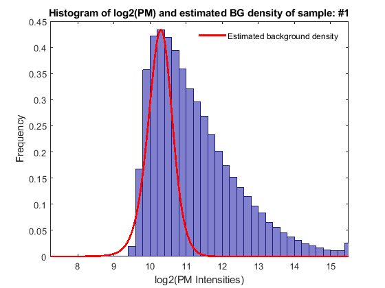
The RMA background adjustment method corrects PM probe intensities chip by chip. The PM probe intensities are modeled as the sum of a normal noise component and an exponential signal component. Use rmabackadj to background adjust the PM intensities in the CNS data. You can inspect the intensity distribution histogram and the estimated background adjustment of a specific chip by setting the input parameter SHOWPLOT to the column index of the chip.
pms_bg = rmabackadj(probeData.PMIntensities, 'showplot', 1);

Several nonlinear normalization methods have been successfully applied to Affymetrix microarray data. The RMA procedure normalizes the probe-level data with a quantile normalization method. Use quantilenorm to normalize the background adjusted PM intensities in the CNS data. Note: If you are interested in a rank-invariant set normalization method, use the affyinvarsetnorm function instead.
pms_bgnorm = quantilenorm(pms_bg);
A median polish procedure is applied to the PM intensities in summarization. To calculate the expression values, use rmasummary to summarize probe intensities of each probe set across multiple chips. The expression values are the probe set intensity summaries on a log-2 scale.
cns_rma_exp = rmasummary(probeData.ProbeIndices, pms_bgnorm);
Using the GCRMA Procedure
The GCRMA procedure adjusts for optical noise and non-specific binding (NSB) taking into account the effect of the stronger bonding of G/C pairs (Naef et al., 2003, Wu et al., 2004). GCRMA uses probe sequence information to estimate probe affinities for computing non-specific binding. The probe affinity is modeled as a sum of the position-dependent base effects. Usually, the probe affinities are estimated from the MM intensities of an NSB experiment. If NSB data is not available, the probe affinities can still be estimated from sequence information and MM probe intensities normalized by the probe set median intensity (Naef et al., 2003).
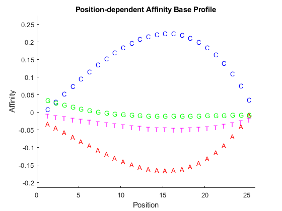
For the CNS dataset, use the data from the microarray hybridized with the normal cerebella sample (Brain_Ncer_1) to compute the probe affinities for the HuGeneFL array. Use affyprobeaffinities to estimate the probe affinities of an Affymetrix microarray. Use the SHOWPLOT input parameter to inspect a plot showing the effects of base A, C, G, and T at the 25 positions.
figure
idx = find(strcmpi('Brain_Ncer_1', samples));
[pmAlpha, mmAlpha] = affyprobeaffinities(S.SequenceMatrix,...
                       probeData.MMIntensities(:, idx), 'showplot', true);

Note: There are 496 probes on a HuGeneFL array that do not have sequence information; the affinities for these probes were NaN.
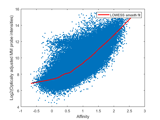
With the probe affinities available, the amount of NSB can be estimated by fitting a LOWESS curve through MM probe intensities vs. MM probe affinities. The function gcrmabackadj performs optical and NSB corrections. The input parameter SHOWPLOT shows a plot of the optical noise adjusted MM intensities against its affinities, and the smooth fit of a specified chip. You can compute the background intensities with one of two estimation methods, Maximum Likelihood Estimate (MLE) and Empirical-Bayes (EB), which computes the posterior mean of specific binding given prior observed intensities. Here you will background adjust four arrays using both estimation methods. (Note: gcrmabackadj will report the progress to the MATLAB command window. You can turn the progress report off by setting the input parameter VERBOSE to false.)
Background adjust the first four chips using GCRMA-MLE method, and inspect the plot of intensity vs. affinity for data from the third array.
pms_MLE_bg = gcrmabackadj(probeData.PMIntensities(:,1:4),...
                            probeData.MMIntensities(:, 1:4),...
                            pmAlpha, mmAlpha, 'showplot', 3);

% Adjust YLIM for better view
ylim([4 16]);
Adjusting background for chip # 1 of 4 using MLE method.
Adjusting background for chip # 2 of 4 using MLE method.
Adjusting background for chip # 3 of 4 using MLE method.
Adjusting background for chip # 4 of 4 using MLE method.

Background adjust the first four chips using the GCRMA-EB method. Processing with this method is more computationally intensive and will take longer.
pms_EB_bg = gcrmabackadj(probeData.PMIntensities(:,1:4),...
                            probeData.MMIntensities(:, 1:4),...
                            pmAlpha, mmAlpha, 'method', 'EB');
Adjusting background for chip # 1 of 4 using EB method.
Adjusting background for chip # 2 of 4 using EB method.
Adjusting background for chip # 3 of 4 using EB method.
Adjusting background for chip # 4 of 4 using EB method.
You can continue the preprocessing with the quatilenorm and rmasummary functions, or use the gcrma function to do everything. The gcrma function performs background adjustment and returns expression measures of background adjusted PM probe intensities using the same normalization and summarization methods as RMA. You can also pass in the sequence matrix instead of affinities. The function will automatically compute the affinities in this case. (Note: gcrma will report the progress to the MATLAB command window. You can turn the progress report off by setting the input parameter VERBOSE to false.)
cns_mle_exp = gcrma(probeData.PMIntensities, probeData.MMIntensities,...
                    probeData.ProbeIndices, pmAlpha, mmAlpha);
Adjusting background for chip # 1 of 42 using MLE method.
Adjusting background for chip # 2 of 42 using MLE method.
Adjusting background for chip # 3 of 42 using MLE method.
Adjusting background for chip # 4 of 42 using MLE method.
Adjusting background for chip # 5 of 42 using MLE method.
Adjusting background for chip # 6 of 42 using MLE method.
Adjusting background for chip # 7 of 42 using MLE method.
Adjusting background for chip # 8 of 42 using MLE method.
Adjusting background for chip # 9 of 42 using MLE method.
Adjusting background for chip # 10 of 42 using MLE method.
Adjusting background for chip # 11 of 42 using MLE method.
Adjusting background for chip # 12 of 42 using MLE method.
Adjusting background for chip # 13 of 42 using MLE method.
Adjusting background for chip # 14 of 42 using MLE method.
Adjusting background for chip # 15 of 42 using MLE method.
Adjusting background for chip # 16 of 42 using MLE method.
Adjusting background for chip # 17 of 42 using MLE method.
Adjusting background for chip # 18 of 42 using MLE method.
Adjusting background for chip # 19 of 42 using MLE method.
Adjusting background for chip # 20 of 42 using MLE method.
Adjusting background for chip # 21 of 42 using MLE method.
Adjusting background for chip # 22 of 42 using MLE method.
Adjusting background for chip # 23 of 42 using MLE method.
Adjusting background for chip # 24 of 42 using MLE method.
Adjusting background for chip # 25 of 42 using MLE method.
Adjusting background for chip # 26 of 42 using MLE method.
Adjusting background for chip # 27 of 42 using MLE method.
Adjusting background for chip # 28 of 42 using MLE method.
Adjusting background for chip # 29 of 42 using MLE method.
Adjusting background for chip # 30 of 42 using MLE method.
Adjusting background for chip # 31 of 42 using MLE method.
Adjusting background for chip # 32 of 42 using MLE method.
Adjusting background for chip # 33 of 42 using MLE method.
Adjusting background for chip # 34 of 42 using MLE method.
Adjusting background for chip # 35 of 42 using MLE method.
Adjusting background for chip # 36 of 42 using MLE method.
Adjusting background for chip # 37 of 42 using MLE method.
Adjusting background for chip # 38 of 42 using MLE method.
Adjusting background for chip # 39 of 42 using MLE method.
Adjusting background for chip # 40 of 42 using MLE method.
Adjusting background for chip # 41 of 42 using MLE method.
Adjusting background for chip # 42 of 42 using MLE method.
Normalizing.
Calculating expression.
Inspecting the Background Adjustment Results
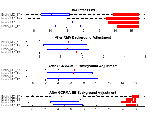
Use boxplots to inspect the PM intensity distributions of the first four chips with three background adjustment procedures.
figure
subplot(4,1,1)
maboxplot(log2(probeData.PMIntensities(:, 1:4)), samples(1:4),...
          'title','Raw Intensities', 'orientation', 'horizontal')
subplot(4,1,2)
maboxplot(log2(pms_bg(:,1:4)), samples(1:4),...
          'title','After RMA Background Adjustment','orient','horizontal')
subplot(4,1,3)
maboxplot(log2(pms_MLE_bg), samples(1:4),...
          'title','After GCRMA-MLE Background Adjustment','orient','horizontal')
subplot(4,1,4)
maboxplot(log2(pms_EB_bg), samples(1:4),...
          'title','After GCRMA-EB Background Adjustment','orient','horizontal')

Use boxplots to inspect the background corrected and normalized PM intensity distributions of the first four chips with three background adjustment procedures.
pms_MLE_bgnorm = quantilenorm(pms_MLE_bg);
pms_EB_bgnorm  = quantilenorm(pms_EB_bg);

figure
subplot(3,1,1)
maboxplot(log2(pms_bgnorm(:, 1:4)), samples(1:4),...
          'title','Normalized RMA Background Adjusted Intensity',...
          'orientation', 'horizontal')
subplot(3,1,2)
maboxplot(log2(pms_MLE_bgnorm), samples(1:4),...
          'title','Normalized GCRMA-MLE Background Adjusted Intensity',...
          'orientation', 'horizontal')
subplot(3,1,3)
maboxplot(log2(pms_EB_bgnorm), samples(1:4),...
          'title','Normalized GCRMA-EB Background Adjusted Intensity',...
          'orientation', 'horizontal')

Final Remarks
You can perform importing of data from CEL files and all three preprocessing steps of the RMA and GCRMA techniques shown in this example by using the affyrma and affygcrma functions respectively.
Affymetrix and GeneChip are registered trademarks of Affymetrix, Inc.
References
[1] Pomeroy, S.L., et al., "Prediction of central nervous system embryonal tumour outcome based on gene expression", Nature, 415(6870):436-42, 2002.
[2] Irizarry, R.A., et al., "Exploration, normalization, and summaries of high density oligonucleotide array probe level data", Biostatistics, 4(2):249-64, 2003.
[3] Wu, Z., et al., "A model based background adjustment for oligonucleotide expression arrays", Journal of the American Statistical Association, 99(468):909-17, 2004.
[4] Bolstad, B.M., et al., "A comparison of normalization methods for high density oligonucleotide array data based on variance and bias", Bioinformatics, 19(2):185-93, 2003.
[5] Naef, F., and Magnasco, M.O. "Solving the riddle of the bright mismatches: labeling and effective binding in oligonucleotide arrays", Physical Review, E, Statistical, Nonlinear and Soft Matter Physics, 68(1Pt1):011906, 2003.


