Visualizing and Preprocessing Hyphenated Mass Spectrometry Data Sets for Metabolite and Protein/Peptide Profiling

Introduction

In a typical hyphenated mass spectrometry experiment, proteins and metabolites are harvested from cells, tissues, or body fluids, dissolved and denatured in solution, and enzymatically digested into mixtures. These mixtures are then separated either by High Performance Liquid Chromatography (HPLC), capillary electrophoresis (CE), or gas chromatography (GC) and coupled to a mass-spectrometry identification method, such as Electrospray Ionization Mass Spectrometry (ESI-MS), matrix assisted ionization (MALDI or SELDI TOF-MS), or tandem mass spectrometry (MS/MS).

Open Data Repositories and mzXML File Format

For this example, we use a test sample LC-ESI-MS data set with a seven protein mix. The data in this example (7MIX_STD_110802_1.mzXML) is not distributed with MATLAB®. To complete this example, you must download a similar data set into a local directory or your own repository. You can try other data sets available in other public databases for protein expression data such as the Peptide Atlas at the Institute of Systems Biology [1].

Most of the current mass spectrometers can translate or save the acquisition data using the mzXML schema. This standard is an XML (eXtensible Markup Language)-based common file format developed by the Sashimi project to address the challenges involved in representing data sets from different manufacturers and from different experimental setups into a common and expandable schema. mzXML files used in hyphenated mass spectrometry are usually very large. The MZXMLINFO function allows you to obtain basic information about the dataset without reading it into memory. For example, you can retrieve the number of scans, the range of the retention time, and the number of tandem MS instruments (levels).

info = mzxmlinfo('7MIX_STD_110802_1.mzXML','NUMOFLEVELS',true)

info = 

  struct with fields:

                            Filename: '7MIX_STD_110802_1.mzXML'
                         FileModDate: '01-Feb-2013 11:54:30'
                            FileSize: 26789612
                       NumberOfScans: 7161
                           StartTime: 'PT0.00683333S'
                             EndTime: 'PT200.036S'
       DataProcessingIntensityCutoff: 'N/A'
            DataProcessingCentroided: 'true'
            DataProcessingDeisotoped: 'N/A'
    DataProcessingChargeDeconvoluted: 'N/A'
       DataProcessingSpotIntegration: 'N/A'
                    NumberOfMSLevels: 2

The MZXMLREAD function reads the XML document into a MATLAB structure. The fields scan and index are placed at the first level of the output structure for improved access to the spectral data. The remainder of the mzXML document tree is parsed according to the schema specifications. This LC/MS data set contains 7161 scans with two MS levels. For this example you will use only the first level scans. Second level spectra are usually used for peptide/protein identification, and come at a later stage in some types of workflow analyses. MZXMLREAD can filter the desired scans without loading all the dataset into memory:

mzXML_struct = mzxmlread('7MIX_STD_110802_1.mzXML','LEVEL',1)

mzXML_struct = 

  struct with fields:

     scan: [2387×1 struct]
    mzXML: [1×1 struct]
    index: [1×1 struct]

If you receive any errors related to memory or java heap space during the loading, try increasing your java heap space as described here.

More detailed information pertaining the mass-spectrometer and the experimental conditions are found in the field msRun.

mzXML_struct.mzXML.msRun

ans = 

  struct with fields:

         scanCount: 7161
         startTime: "PT0.00683333S"
           endTime: "PT200.036S"
        parentFile: [1×1 struct]
      msInstrument: [1×1 struct]
    dataProcessing: [1×1 struct]

To facilitate the handling of the data, the MZXML2PEAKS function extracts the list of peaks from each scan into a cell array (peaks]) and their respective retention time into a column vector (time). You can extract the spectra of certain level by setting the LEVEL input parameter.

[peaks,time] = mzxml2peaks(mzXML_struct);
numScans = numel(peaks)

numScans =

        2387

The MSDOTPLOT function creates an overview display of the most intense peaks in the entire data set. In this case, we visualize only the most intense 5% ion intensity peaks by setting the input parameter QUANTILE to 0.95.

h = msdotplot(peaks,time,'quantile',.95);
title('5 Percent Overall Most Intense Peaks')

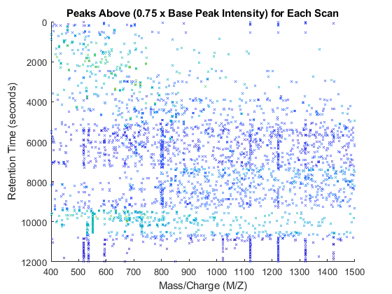
You can also filter the peaks individually for each scan using a percentile of the base peak intensity. The base peak is the most intense peak found in each scan [2]. This parameter is given automatically by most of the spectrometers. This operation requires querying into the mxXML structure to obtain the base peak information. Note that you could also find the base peak intensity by iterating the MAX function over the peak list.

basePeakInt = [mzXML_struct.scan.basePeakIntensity]';
peaks_fil = cell(numScans,1);
for i = 1:numScans
    h = peaks{i}(:,2) > (basePeakInt(i).*0.75);
    peaks_fil{i} = peaks{i}(h,:);
end

whos('basePeakInt','level_1','peaks','peaks_fil')
msdotplot(peaks_fil,time)
title('Peaks Above (0.75 x Base Peak Intensity) for Each Scan')

  Name                Size               Bytes  Class     Attributes

  basePeakInt      2387x1                19096  double              
  peaks            2387x1             14069992  cell                
  peaks_fil        2387x1               327760  cell                

You can customize a 3-D overview of the filtered peaks using the STEM3 function. The STEM3 function requires to put the data into three vectors, whose elements form the triplets (the retention time, the mass/charge, and the intensity value) that represent every stem.

peaks_3D = cell(numScans,1);
for i = 1:numScans
    peaks_3D{i}(:,[2 3]) = peaks_fil{i};
    peaks_3D{i}(:,1) = time(i);
end
peaks_3D = cell2mat(peaks_3D);

figure
stem3(peaks_3D(:,1),peaks_3D(:,2),peaks_3D(:,3),'marker','none')
axis([0 12000 400 1500 0 1e9])
view(60,60)
xlabel('Retention Time (seconds)')
ylabel('Mass/Charge (M/Z)')
zlabel('Relative Ion Intensity')
title('Peaks Above (0.75 x Base Peak Intensity) for Each Scan')

You can plot colored stems using the PATCH function. For every triplet in peaks_3D, interleave a new triplet with the intensity value set to zero. Then create a color vector dependent on the intensity of the stem. A logarithmic transformation enhances the dynamic range of the colormap. For the interleaved triplets assign a NaN, so that PATCH function does not draw lines connecting contiguous stems.

peaks_patch = sortrows(repmat(peaks_3D,2,1));
peaks_patch(2:2:end,3) = 0;

col_vec = log(peaks_patch(:,3));
col_vec(2:2:end) = NaN;

figure
patch(peaks_patch(:,1),peaks_patch(:,2),peaks_patch(:,3),col_vec,...
      'edgeColor','flat','markeredgecolor','flat','Marker','x','MarkerSize',3);
axis([0 12000 400 1500 0 1e9])
view(90,90)
xlabel('Retention Time (seconds)')
ylabel('Mass/Charge (M/Z)')
zlabel('Relative Ion Intensity')
title('Peaks Above (0.75 x Base Peak Intensity) for Each Scan')

view(40,40)

Creating Heat Maps of LC/MS Data Sets

Common techniques in the industry work with peak information (a.k.a. centroided data) instead of raw signals. This may save memory, but some important details are not visible, especially when it is necessary to inspect samples with complex mixtures. To further analyze this data set, we can create a common grid in the mass/charge dimension. Since not all of the scans have enough information to reconstruct the original signal, we use a peak preserving resampling method. By choosing the appropriate parameters for the MSPPRESAMPLE function, you can ensure that the resolution of the spectra is not lost, and that the maximum values of the peaks correlate to the original peak information.

[MZ,Y] = msppresample(peaks,5000);
whos('MZ','Y')

  Name         Size                 Bytes  Class     Attributes

  MZ        5000x1                  20000  single              
  Y         5000x2387            47740000  single              

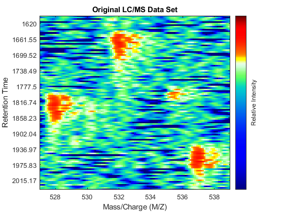
With this matrix of ion intensities, Y, you can create a colored heat map. The MSHEATMAP function automatically adjusts the colorbar utilized to show the statistically significant peaks with hot colors and the noisy peaks with cold colors. The algorithm is based on clustering significant peaks and noisy peaks by estimating a mixture of Gaussians with an Expectation-Maximization approach. Additionally, you can use the MIDPOINT input parameter to select an arbitrary threshold to separate noisy peaks from significant peaks, or you can interactively shift the colormap to hide or unhide peaks. When working with heat maps, it is common to display the logarithm of the ion intensities, which enhances the dynamic range of the colormap.

fh1 = msheatmap(MZ,time,log(Y),'resolution',.1,'range',[500 900]);
title('Original LC/MS Data Set')

You can zoom to small regions of interest to observe the data, either interactively or programmatically using the AXIS function. We observe some regions with high relative ion intensity. These represent peptides in the biological sample.

axis([527 539 385 496])

You can overlay the original peak information of the LC/MS data set. This lets you evaluate the performance of the peak-preserving resampling operation. You can use the returned handle to hide/unhide the dots.

dp1 = msdotplot(peaks,time);

Calibrating the Mass/Charge Location of Peaks to a Common Grid

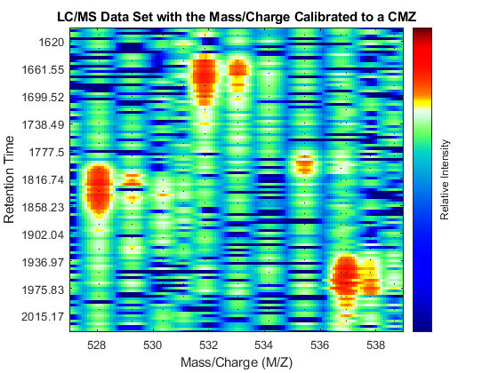
The two dimensional peaks appear to be noisy or they do not show a compact shape in contiguous spectra. This is a common problem for many mass spectrometers. Random fluctuations of the mass/charge value extracted from peaks of replicate profiles are reported to range from 0.1% to 0.3% [3]. Such variability can be caused by several factors, e.g. poor calibration of the detector, low signal-to-noise ratio, or problems in the peak extraction algorithms. The MSPALIGN function implements advanced data binning algorithms that synchronize all the spectra in a data set to a common mass/charge grid (CMZ). CMZ can be chosen arbitrarily or it can be estimated after analyzing the data [2,4,5]. The peak matching procedure can use either a nearest neighbor rule or a dynamic programming alignment.

[CMZ, peaks_CMZ] = mspalign(peaks);

Repeat the visualization process with the aligned peaks: perform peak preserving resampling, create a heat map, overlay the aligned peak information, and zoom into the same region of interest as before. When the spectrum is re-calibrated, it is possible to distinguish the isotope patterns of some of the peptides.

[MZ_A,Y_A] = msppresample(peaks_CMZ,5000);
fh2 = msheatmap(MZ_A,time,log(Y_A),'resolution',.10,'range',[500 900]);
title('LC/MS Data Set with the Mass/Charge Calibrated to a CMZ')
dp2 = msdotplot(peaks_CMZ,time);
axis([527 539 385 496])

Calibrating the Mass/Charge Location of Peaks Locally

MSPALIGN computes a single CMZ for the whole LC/MS data set. This may not be the ideal case for samples with more complex mixtures of peptides and/or metabolites than the data set utilized in this example. In the case of complex mixtures, you can align each spectrum to a local set of spectra that contain only informative peaks (high intensity) with similar retention times, otherwise the calibration process in regions with small peaks (low intensity) can be biased by other peaks that share similar mass/charge values but are at different retention times. To perform a finer calibration, you can employ the SAMPLEALIGN function. This function is a generalization of the Constrained Dynamic Time Warping (CDTW) algorithms commonly utilized in speech processing [6]. In the following for loop, we maintain a buffer with the intensities of the previous aligned spectra (LAI). The ion intensities of the spectra are scaled with the anonymous function SF (inside SAMPLEALIGN) to reduce the distance between large peaks. SAMPLEALIGN reduces the overall distance of all matched points and introduces gaps as necessary. In this case we use a finer MZ vector (FMZ), such that we preserve the correct value of the mass/charge of the peaks as much as possible. Note: this may take some time, as the CDTW algorithm is executed 2,387 times.

SF = @(x) 1-exp(-x./5e7); % scaling function
DF = @(R,S) sqrt((SF(R(:,2))-SF(S(:,2))).^2 + (R(:,1)-S(:,1)).^2);

FMZ = (500:0.15:900)';  % setup a finer MZ vector
LAI = zeros(size(FMZ)); % init buffer for the last alignment intensities

peaks_FMZ = cell(numScans,1);
for i = 1:numScans
    % show progress
    if ~rem(i,250)
        fprintf(' %d...',i);
    end
    % align peaks in current scan to LAI
    [k,j] = samplealign([FMZ,LAI],double(peaks{i}),'band',1.5,'gap',[0,2],'dist',DF);
    % updating the LAI buffer
    LAI = LAI*.25;
    LAI(k) = LAI(k) + peaks{i}(j,2);
    % save the alignment
    peaks_FMZ{i} = [FMZ(k) peaks{i}(j,2)];
end

 250... 500... 750... 1000... 1250... 1500... 1750... 2000... 2250...

Repeat the visualization process and zoom to the region of interest.

[MZ_B,Y_B] = msppresample(peaks_FMZ,4000);
fh3 = msheatmap(MZ_B,time,log(Y_B),'resolution',.10,'range',[500 900]);
title('LC/MS Data Set with the Mass/Charge Calibrated Locally')
dp3 = msdotplot(peaks_FMZ,time);
axis([527 539 385 496])

As a final step to improve the image, you can apply a Gaussian filter in the chromatographic direction to smooth the whole data set.

Gpulse = exp(-.1*(-10:10).^2)./sum(exp(-.1*(-10:10).^2));
YF = convn(Y_B,Gpulse,'same');
fh4 = msheatmap(MZ_B,time,log(YF),'resolution',.10,'limits',[500 900]);
title('Final Enhanced LC/MS Data Set')
dp4 = msdotplot(peaks_FMZ,time);
axis([527 539 385 496])

You can link the axes of two heat maps, to interactively or programmatically compare regions between two data sets. In this case we compare the original and the final enhanced LC/MS matrices.

linkaxes(findobj([fh1 fh4],'Tag','MSHeatMap'))
axis([521 538 266 617])

Extracting Spectra Using the Total Ion Chromatogram

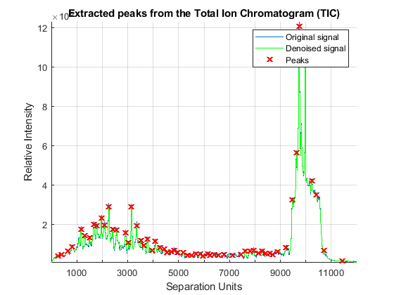
Once the LC/MS data set is smoothed and resampled into a regular grid, it is possible to extract the most informative spectra by looking at the local maxima of the Total Ion Chromatogram (TIC). The TIC is straightforwardly computed by summing the rows of YF. Then, use the MSPEAKS function to find the retention time values for extracting selected subsets of spectra.

TIC = mean(YF);
pt = mspeaks(time,TIC','multiplier',10,'overseg',100,'showplot',true);
title('Extracted peaks from the Total Ion Chromatogram (TIC)')
pt(pt(:,1)>4000,:) = []; % remove spectra above 4000 seconds
numPeaks = size(pt,1)

numPeaks =

    22

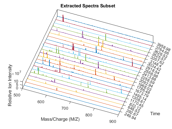
Create a 3-D plot of the selected spectra.

xRows = samplealign(time,pt(:,1),'width',1); % finds the time index for every peak
xSpec = YF(:,xRows);                         % gets the signals to plot

figure;
hold on
box on
plot3(repmat(MZ_B,1,numPeaks),repmat(1:numPeaks,numel(MZ_B),1),xSpec)
view(20,85)

ax = gca;
ax.YTick = 1:numPeaks;
ax.YTickLabel = num2str(time(xRows));
axis([500 900 0 numPeaks 0 1e8])

xlabel('Mass/Charge (M/Z)')
ylabel('Time')
zlabel('Relative Ion Intensity')
title('Extracted Spectra Subset')

Overlay markers for the extracted spectra over the enhanced heatmap.

linkaxes(findobj(fh4,'Tag','MSHeatMap'),'off')
figure(fh4)
hold on
for i = 1:numPeaks
    plot([400 1500],xRows([i i]),'m')
end
axis([500 900 100 925])
dp4.Visible = 'off';
title('Final Enhanced LC/MS Data Set with Extracted Spectra Marked')

References

[1] Desiere, F. et al., "The Peptide Atlas Project", Nucleic Acids Research, 34:D655-8, 2006.

[2] Purvine, S., Kolker, N., and Kolker, E., "Spectral Quality Assessment for High-Throughput Tandem Mass Spectrometry Proteomics", OMICS: A Journal of Integrative Biology, 8(3):255-65, 2004.

[3] Kazmi, A.S., et al., "Alignment of high resolution mass spectra: Development of a heuristic approach for metabolomics", Metabolomics, 2(2):75-83, 2006.

[4] Jeffries, N., "Algorithms for alignment of mass spectrometry proteomic data", Bioinformatics, 21(14):3066-3073, 2005.

[5] Yu, W., et al., "Multiple peak alignment in sequential data analysis: A scale-space based approach", IEEE®/ACM Trans. Computational Biology and Bioinformatics, 3(3):208-219, 2006.

[6] Sakoe, H. and Chiba s., "Dynamic programming algorithm optimization for spoken word recognition", IEEE Trans. Acoustics, Speech and Signal Processing, ASSP-26(1):43-9, 1978.