Use Generated Code to Accelerate an Application Deployed with MATLAB Compiler
This example shows how to use generated code to accelerate an application that you deploy with MATLAB® Compiler™. The example accelerates an algorithm by using MATLAB® Coder™ to generate a MEX version of the algorithm. It uses MATLAB Compiler to deploy a standalone application that calls the MEX function. The deployed application uses the MATLAB® Runtime which enables royalty-free deployment to someone who does not have MATLAB®.
This workflow is useful when:
You want to deploy an application to a platform that the MATLAB Runtime supports.
The application includes a computationally intensive algorithm that is suitable for code generation.
The generated MEX for the algorithm is faster than the original MATLAB algorithm.
You do not need to deploy readable C/C++ source code for the application.
The example application uses a DSP algorithm that requires the DSP System Toolbox™.
Create the MATLAB Application
For acceleration, it is a best practice to separate the computationally intensive algorithm from the code that calls it.
In this example, myRLSFilterSystemIDSim implements the algorithm. myRLSFilterSystemIDApp provides a user interface that calls myRLSFilterSystemIDSim.
myRLSFilterSystemIDSim simulates system identification by using recursive least-squares (RLS) adaptive filtering. The algorithm uses dsp.VariableBandwidthFIRFilter to model the unidentified system and dsp.RLSFilter to identify the FIR filter.
myRLSFilterSystemIDApp provides a user interface that you use to dynamically tune simulation parameters. It runs the simulation for a specified number of time steps or until you stop the simulation. It plots the results of the simulation on scopes.
For details about this application, see System Identification Using RLS Adaptive Filtering (DSP System Toolbox) in the DSP System Toolbox documentation.
In a writable folder, create myRLSFilterSystemIDSim and myRLSFilterSystemIDApp. Alternatively, to access these files, click Open Script.
myRLSFilterSystemIDSim
function [tfe,err,cutoffFreq,ff] = ...
    myRLSFilterSystemIDSim(tuningUIStruct)
% myRLSFilterSystemIDSim implements the algorithm used in
% myRLSFilterSystemIDApp.
% This function instantiates, initializes, and steps through the System
% objects used in the algorithm.
%
% You can tune the cutoff frequency of the desired system and the
% forgetting factor of the RLS filter through the GUI that appears when
% myRLSFilterSystemIDApp is executed.

%   Copyright 2013-2017 The MathWorks, Inc.

%#codegen

% Instantiate and initialize System objects. The objects are declared
% persistent so that they are not recreated every time the function is
% called inside the simulation loop.
persistent rlsFilt sine unknownSys transferFunctionEstimator
if isempty(rlsFilt)
    % FIR filter models the unidentified system
    unknownSys = dsp.VariableBandwidthFIRFilter('SampleRate',1e4,...
        'FilterOrder',30,...
        'CutoffFrequency',.48 * 1e4/2);
    % RLS filter is used to identify the FIR filter
    rlsFilt = dsp.RLSFilter('ForgettingFactor',.99,...
        'Length',28);
    % Sine wave used to generate input signal
    sine = dsp.SineWave('SamplesPerFrame',1024,...
        'SampleRate',1e4,...
        'Frequency',50);
    % Transfer function estimator used to estimate frequency responses of
    % FIR and RLS filters.
    transferFunctionEstimator = dsp.TransferFunctionEstimator(...
        'FrequencyRange','centered',...
        'SpectralAverages',10,...
        'FFTLengthSource','Property',...
        'FFTLength',1024,...
        'Window','Kaiser');
end

if tuningUIStruct.Reset
    % reset System objects
    reset(rlsFilt);
    reset(unknownSys);
    reset(transferFunctionEstimator);
    reset(sine);
end

% Tune FIR cutoff frequency and RLS forgetting factor
if  tuningUIStruct.ValuesChanged
    param = tuningUIStruct.TuningValues;
    unknownSys.CutoffFrequency  = param(1);
    rlsFilt.ForgettingFactor = param(2);
end

% Generate input signal - sine wave plus Gaussian noise
inputSignal = sine() +  .1 * randn(1024,1);

% Filter input though FIR filter
desiredOutput = unknownSys(inputSignal);

% Pass original and desired signals through the RLS Filter
[rlsOutput , err] = rlsFilt(inputSignal,desiredOutput);

% Prepare system input and output for transfer function estimator
inChans = repmat(inputSignal,1,2);
outChans = [desiredOutput,rlsOutput];

% Estimate transfer function
tfe = transferFunctionEstimator(inChans,outChans);

% Save the cutoff frequency and forgetting factor
cutoffFreq = unknownSys.CutoffFrequency;
ff = rlsFilt.ForgettingFactor;

end
myRLSFilterSystemIDApp
function scopeHandles = myRLSFilterSystemIDApp(numTSteps)
% myRLSFilterSystemIDApp initialize and execute RLS Filter
% system identification example. Then, display results using
% scopes. The function returns the handles to the scope and UI objects.
%
% Input:
%   numTSteps - number of time steps
% Outputs:
%   scopeHandles    - Handle to the visualization scopes

% Copyright 2013-2017 The MathWorks, Inc.


if nargin == 0
    numTSteps = Inf; % Run until user stops simulation.
end

% Create scopes
tfescope = dsp.ArrayPlot('PlotType','Line',...
    'Position',[8 696 520 420],...
    'YLimits',[-80 30],...
    'SampleIncrement',1e4/1024,...
    'YLabel','Amplitude (dB)',...
    'XLabel','Frequency (Hz)',...
    'Title','Desired and Estimated Transfer Functions',...
    'ShowLegend',true,...
    'XOffset',-5000);

msescope = timescope('SampleRate',1e4,...
    'Position',[8 184 520 420],...
    'TimeSpanSource','property','TimeSpan',0.01,...
    'YLimits',[-300 10],'ShowGrid',true,...
    'YLabel','Mean-Square Error (dB)',...
    'Title','RLSFilter Learning Curve');

screen = get(0,'ScreenSize');
outerSize = min((screen(4)-40)/2, 512);
tfescope.Position = [8, screen(4)-outerSize+8, outerSize+8,...
    outerSize-92];
msescope.Position = [8, screen(4)-2*outerSize+8, outerSize+8, ...
    outerSize-92];

% Create UI to tune FIR filter cutoff frequency and RLS filter
%  forgetting factor
Fs = 1e4;
param = struct([]);
param(1).Name = 'Cutoff Frequency (Hz)';
param(1).InitialValue = 0.48 * Fs/2;
param(1).Limits = Fs/2 * [1e-5, .9999];
param(2).Name = 'RLS Forgetting Factor';
param(2).InitialValue = 0.99;
param(2).Limits = [.3, 1];
hUI = HelperCreateParamTuningUI(param, 'RLS FIR Demo');
set(hUI,'Position',[outerSize+32, screen(4)-2*outerSize+8, ...
    outerSize+8, outerSize-92]);

% Execute algorithm
while(numTSteps>=0)

    S = HelperUnpackUIData(hUI);

    drawnow limitrate;   % needed to process UI callbacks

    [tfe,err] = myRLSFilterSystemIDSim(S);

    if S.Stop     % If "Stop Simulation" button is pressed
        break;
    end
    if S.Pause
        continue;
    end

    % Plot transfer functions
    tfescope(20*log10(abs(tfe)));
    % Plot learning curve
    msescope(10*log10(sum(err.^2)));
    numTSteps = numTSteps - 1;
end

if ishghandle(hUI)  % If parameter tuning UI is open, then close it.
    delete(hUI);
    drawnow;
    clear hUI
end

scopeHandles.tfescope = tfescope;
scopeHandles.msescope = msescope;
end
Test the MATLAB Application
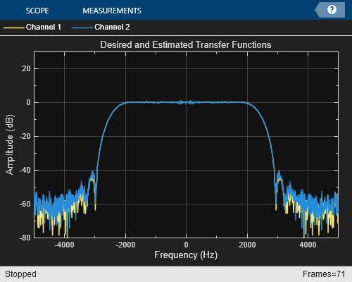
Run the system identification application for 100 time steps. The application runs the simulation for 100 time steps or until you click Stop Simulation. It plots the results on scopes.
scope1 = myRLSFilterSystemIDApp(100);
release(scope1.tfescope);
release(scope1.msescope);

Prepare Algorithm for Acceleration
When you use MATLAB Coder to accelerate a MATLAB algorithm, the code must be suitable for code generation.
1. Make sure that myRLSFilterSystemIDSim.m includes the %#codegen directive after the function signature.
This directive indicates that you intend to generate code for the function. In the MATLAB Editor, it enables the code analyzer to detect code generation issues.
2. Screen the algorithm for unsupported functions or constructs.
coder.screener('myRLSFilterSystemIDSim');
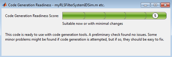
The code generation readiness tool does not find code generation issues in this algorithm.
Accelerate the Algorithm
To accelerate the algorithm, this example use the MATLAB Coder codegen command. Alternatively, you can use the MATLAB Coder app. For code generation, you must specify the type, size, and complexity of the input arguments. The function myRLSFilterSystemIDSim takes a structure that stores tuning information. Define an example tuning structure and pass it to codegen by using the -args option.
ParamStruct.TuningValues = [2400 0.99];
ParamStruct.ValuesChanged = false;
ParamStruct.Reset = false;
ParamStruct.Pause = false;
ParamStruct.Stop  = false;
codegen myRLSFilterSystemIDSim -args {ParamStruct};
Code generation successful.
codegen creates the MEX function myRLSFilterSystemIDSim_mex in the current folder.
Compare MEX Function and MATLAB Function Performance
1. Time 100 executions of myRLSFilterSystemIDSim.
clear myRLSFilterSystemIDSim
disp('Running the MATLAB function ...')
tic
nTimeSteps = 100;
for ind = 1:nTimeSteps
     myRLSFilterSystemIDSim(ParamStruct);
end
tMATLAB = toc;
Running the MATLAB function ...
2. Time 100 executions of myRLSFilterSystemIDSim_mex.
clear myRLSFilterSystemIDSim
disp('Running the MEX function ...')
tic
for ind = 1:nTimeSteps
    myRLSFilterSystemIDSim_mex(ParamStruct);
end
tMEX = toc;

disp('RESULTS:')
disp(['Time for original MATLAB function: ', num2str(tMATLAB),...
     ' seconds']);
disp(['Time for MEX function: ', num2str(tMEX), ' seconds']);
disp(['The MEX function is ', num2str(tMATLAB/tMEX),...
    ' times faster than the original MATLAB function.']);
Running the MEX function ...
RESULTS:
Time for original MATLAB function: 0.44044 seconds
Time for MEX function: 0.093679 seconds
The MEX function is 4.7016 times faster than the original MATLAB function.
Optimize the MEX code
You can sometimes generate faster MEX by using a different C/C++ compiler or by using certain options or optimizations. See Accelerate MATLAB Algorithms.
For this example, the MEX is sufficiently fast without further optimization.
Modify the Application to Call the MEX Function
Modify myRLSFilterSystemIDApp so that it calls myRLSFilterSystemIDSim_mex instead of myRLSFilterSystemIDSim.
Save the modified function in myRLSFilterSystemIDApp_acc.m.
Test the Application with the Accelerated Algorithm
clear myRLSFilterSystemIDSim_mex;
scope2 = myRLSFilterSystemIDApp_acc(100);
release(scope2.tfescope);
release(scope2.msescope);
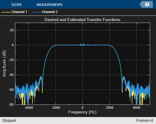
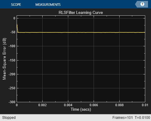
The behavior of the application that calls the MEX function is the same as the behavior of the application that calls the original MATLAB function. However, the plots update more quickly because the simulation is faster.
Create the Standalone Application
1. To open the Application Compiler App, on the Apps tab, under Application Deployment, click the app icon.
2. Specify that the main file is myRLSFilterSystemIDApp_acc.
The app determines the required files for this application. The app can find the MATLAB files and MEX-files that an application uses. You must add other types of files, such as MAT files or images, as required files.
3. In the Packaging Options section of the toolstrip, make sure that the Runtime downloaded from web check box is selected.
This option creates an application installer that downloads and installs the MATLAB Runtime with the deployed MATLAB application.
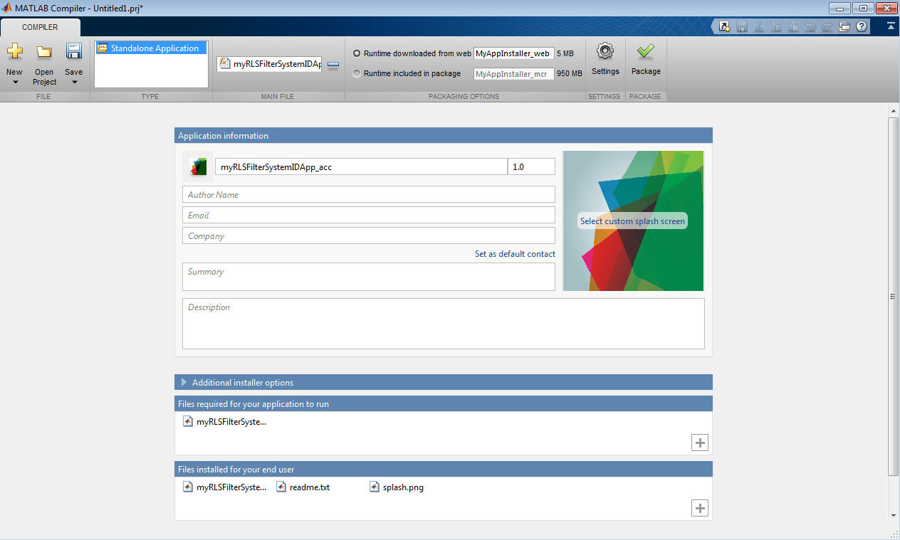
4. Click Package and save the project.
5. In the Package window, make sure that the Open output folder when process completes check box is selected.
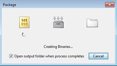
When the packaging is complete, the output folder opens.
Install the Application
1. Open the for_redistribution folder.
2. Run MyAppInstaller_web.
3. If you connect to the internet by using a proxy server, enter the server settings.
4. Advance through the pages of the installation wizard.
On the Installation Options page, use the default installation folder.
On the Required Software page, use the default installation folder.
On the License agreement page, read the license agreement and accept the license.
On the Confirmation page, click Install.
If the MATLAB Runtime is not already installed, the installer installs it.
5. Click Finish.
Run the Application
1. Open a terminal window.
2. Navigate to the folder where the application is installed.
For Windows®, navigate to
C:\Program Files\myRLSFilterSystemIDApp_acc.For macOS, navigate to
/Applications/myRLSFilterSystemIDApp_acc.For Linux®, navigate to
/usr/myRLSFilterSystemIDApp_acc.
3. Run the application by using the appropriate command for your platform.
For Windows, use
application\myRLSFilterSystemIDApp_acc.For macOS, use
myRLSFilterSystemIDApp_acc.app/Contents/MacOS/myRLSFilterSystemIDApp_acc.For Linux, use
/myRLSFilterSystemIDApp_acc.
Starting the application takes approximately the same amount of time as starting MATLAB.