Simultaneous Simulation of Multiple Fading Channels with WINNER II Channel Model

Check for Support Package Installation

Check if the 'WINNER II Channel Model for Communications Toolbox' support package is installed.

commSupportPackageCheck("CST_WINNER2");

Antenna Array Inventory

In the WINNER II channel model, each BS is composed of one or more sectors, and each BS sector and MS is assigned with an antenna array. We need to first establish a set of arrays that are available for BS sectors and MS to employ, which we call the antenna array inventory.

In this example, all available antenna arrays are uniform circular array (UCA). There are four different UCAs in the inventory:

Each antenna element in the UCAs is omnidirectional.

s = rng(21); % For repeatability

AA(1) = winner2.AntennaArray("UCA",16,0.3);
AA(2) = winner2.AntennaArray("UCA",12,0.3);
AA(3) = winner2.AntennaArray("UCA",8,0.3);
AA(4) = winner2.AntennaArray("UCA",4,0.05);

Configure System Layout

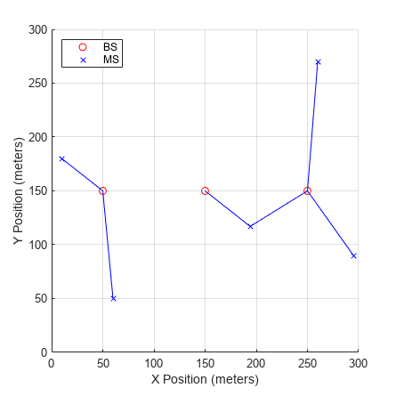
On a 300-by-300 (meters) map, we will set up 3 BS, 5 MS, and 6 links. The first BS has one sector which is equipped with a 16-element UCA. The second BS also has one sector that is equipped with a 12-element UCA. The third BS has three sectors which are equipped with a 8-element UCA each. Each MS is assigned with a 4-element UCA.

BSIdx = {1; 2; [3 3 3]}; % Index in antenna array inventory vector
MSIdx = [4 4 4 4 4];     % Index in antenna array inventory vector
numLinks = 6;            % Number of links
range = 300;             % Layout range (meters)
cfgLayout = winner2.layoutparset(MSIdx,BSIdx,numLinks,AA,range);

Six links are modeled in the system. The first BS connects to the first and second MSs. The second BS connects to the third MS. For the third BS, its first sector connects to the third and fourth MSs, its second sector connects to the fifth MS, and its third sector does not connect to any MS. From MS perspective, each of them connects to one BS except for the third one, which connects to both the second and third BSs. Each link is assigned with one propagation scenario, chosen from B4 (outdoor to indoor), C2 (Urban macro-cell) and C4 (Urban macro outdoor to indoor). Non-line-of-sight (NLOS) is modeled for each link.

cfgLayout.Pairing = [1 1 2 3 3 4; 6 7 8 8 9 10];  % Index in cfgLayout.Stations
cfgLayout.ScenarioVector = [6 6 13 13 11 11];     % 6 for B4, 11 for C2 and 13 for C4
cfgLayout.PropagConditionVector = [0 0 0 0 0 0];  % 0 for NLOS

The three BSs are uniformly spaced between 0 and 300 on the x-axis and have the same position on the y-axis. MS positions are assigned to ensure that their distances to the connected BSs are in the valid path loss ranges for the corresponding scenarios. Specifically, the ranges for the B4, C2 and C4 scenarios are [3, 1000], [50, 5000] and [50, 5000] meters, respectively. By default, each BS sector is 32 meters high and MS is 1.5 meters high. Each MS is randomly assigned with a velocity which does not exceed 0.5 m/s in any of the X, Y and Z directions.

% Number of BS sectors and MSs in the system
numBSSect = sum(cfgLayout.NofSect);
numMS = length(MSIdx);

% Set up positions for BS sectors. Same position for the 
% third, fourth and fifth sectors as they belong to one BS.
cfgLayout.Stations(1).Pos(1:2) = [50;  150];
cfgLayout.Stations(2).Pos(1:2) = [150; 150];
cfgLayout.Stations(3).Pos(1:2) = [250; 150];
cfgLayout.Stations(4).Pos(1:2) = [250; 150];
cfgLayout.Stations(5).Pos(1:2) = [250; 150];

% Set up MS positions
cfgLayout.Stations(6).Pos(1:2) = [10;  180]; % 50m from 1st BS
cfgLayout.Stations(7).Pos(1:2) = [60;  50];  % 111.8m from 1st BS
cfgLayout.Stations(8).Pos(1:2) = [194; 117]; % 55m and 65m from 2nd and 3rd BSs respectively
cfgLayout.Stations(9).Pos(1:2) = [260; 270]; % 120.4m from 3rd BS
cfgLayout.Stations(10).Pos(1:2) = [295; 90]; % 75m from 3rd BS

% Randomly draw MS velocity
for i = numBSSect + (1:numMS)
    cfgLayout.Stations(i).Velocity = rand(3,1) - 0.5;
end

To illustrate the system setup, we plot the BSs, the MSs, and the links between them on a 2-D map. In the plot, each BS sector is represented by a circle, each MS is represented by a cross, and each link is represented by a straight line between the corresponding BS and MS. As the third BS has three sectors, only three circles are shown on the map.

% Get all BS sector and MS positions
BSPos = cell2mat({cfgLayout.Stations(1:numBSSect).Pos});
MSPos = cell2mat({cfgLayout.Stations(numBSSect+1:end).Pos});

scrsz = get(groot,"ScreenSize");
figSize = min(scrsz([3,4]))/2.3;
figure( ...
    Position=[scrsz(3)*.5-figSize/2,scrsz(4)*.7-figSize/2,figSize,figSize]);
hold on; 
grid on;
hBS = plot(BSPos(1,:),BSPos(2,:),"or");   % Plot BS
hMS = plot(MSPos(1,:),MSPos(2,:),"xb");   % Plot MS
for linkIdx = 1:numLinks                  % Plot links
    pairStn = cfgLayout.Pairing(:,linkIdx);
    pairPos = cell2mat({cfgLayout.Stations(pairStn).Pos});
    plot(pairPos(1,:),pairPos(2,:),"-b");
end
xlim([0 300]); ylim([0 300]);
xlabel("X Position (meters)");
ylabel("Y Position (meters)")
legend([hBS, hMS],"BS","MS",location="northwest");

Configure Model Parameters

There are multiple model parameters that can be adjusted in the structure created by the winner2.wimparset function. In this example, the center frequency is 5.25 GHz. Path loss and shadowing fading are modeled for each link. To support bandwidth up to 100 MHz, the two strongest clusters of each link are divided into 3 subclusters each which are 5 ns apart. All links are sampled at different rates which depend on the velocity of the MSs. Because the third and fourth links connect to the same MS, they share the same sample rate.

frameLen = 1600; % Number of samples to be generated

cfgWim = winner2.wimparset;
cfgWim.NumTimeSamples = frameLen;
cfgWim.IntraClusterDsUsed = "yes";
cfgWim.CenterFrequency = 5.25e9;
cfgWim.UniformTimeSampling = "no";
cfgWim.ShadowingModelUsed = "yes";
cfgWim.PathLossModelUsed = "yes";
cfgWim.RandomSeed = 31415926;       % For repeatability

Create WINNER II Channel System Object™

We are now able to use the model and layout configurations to create a WINNER II channel System object. Once the object is created, you can call its info method to view some derived system parameters. For example, in the info method return, the NumBSElements, NumMSElements and NumPaths fields indicate the number of array elements at BS sectors, the number of array elements at MSs and the number of paths for each link. The SampleRate field also shows the sample rate for each link.

WINNERChan = comm.WINNER2Channel(cfgWim,cfgLayout);
chanInfo = info(WINNERChan)

chanInfo = struct with fields:
               NumLinks: 6
          NumBSElements: [16 16 12 8 8 8]
          NumMSElements: [4 4 4 4 4 4]
               NumPaths: [16 16 16 16 24 24]
             SampleRate: [3.0636e+07 3.5303e+07 2.7559e+07 2.7559e+07 3.9688e+07 4.3108e+07]
     ChannelFilterDelay: [7 7 7 7 7 7]
    NumSamplesProcessed: 0

Process Impulse Signal for Each Link

We pass an impulse signal through each link and observe the impulse and frequency responses at the MS. To do so, we need to create the impulse signal for each link and aggregate them into a cell array. This is achieved by using the NumBSElements field of the info method return and the cellfun function. The impulse signal cell array is to be processed by the channel object.

txSig = cellfun(@(x) [ones(1,x);zeros(frameLen-1,x)], ...
    num2cell(chanInfo.NumBSElements)',UniformOutput=false);

rxSig = WINNERChan(txSig); % Pass impulse signal through each link

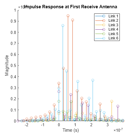
Plotting the received signal at MSs gives an idea about how the fading channel's impulse and frequency responses look for each link. Out of the 4 antennas at each MS, only the received signal at the first antenna is plotted. The fact that the links are sampled at different rates is captured in the impulse response plot. For each link, the first few samples from a channel filter delay are plotted in the negative time axis, if any.

figure(Position= ...
    [scrsz(3)*.3-figSize/2,scrsz(4)*.25-figSize/2,figSize,figSize]);
hold on;
for linkIdx = 1:numLinks
    delay = chanInfo.ChannelFilterDelay(linkIdx);
    stem(((0:(frameLen-1))-delay)/chanInfo.SampleRate(linkIdx), ...
        abs(rxSig{linkIdx}(:,1)));
end
maxX = max((cell2mat(cellfun(@(x) find(abs(x) < 1e-8,1,"first"), ...
    rxSig.',UniformOutput=false)) - chanInfo.ChannelFilterDelay)./ ...
    chanInfo.SampleRate);
minX = -max(chanInfo.ChannelFilterDelay./chanInfo.SampleRate);
xlim([minX, maxX]);
xlabel("Time (s)"); 
ylabel("Magnitude");
legend("Link 1","Link 2","Link 3","Link 4","Link 5","Link 6");
title("Impulse Response at First Receive Antenna");

As the third and fourth links connect to the same MS and hence have the same sample rate, we plot them together using the Spectrum Analyzer System object. The two links have 16 paths each and demonstrate significant frequency selectivity.

sa = spectrumAnalyzer( ...
    Name="Frequency response", ...
    Method="welch", ...
    SpectrumType="power-density", ...
    SampleRate=chanInfo.SampleRate(3), ...
    Position=[scrsz(3)*.7-figSize/2,scrsz(4)*.25-figSize/2,figSize,figSize], ...
    Title="Frequency Response", ...
    ShowLegend=true, ...
    ChannelNames=["Link 3","Link 4"]);

sa(cell2mat(cellfun(@(x) x(:,1),rxSig(3:4,1)',UniformOutput=false)));
release(sa)

rng(s); % Restore RNG

Further Exploration

The example shows how to configure a WINNER II fading channel System object to model a system with multiple MIMO links from BSs to MSs. Further exploration includes modifications to the fields of the cfgLayout and cfgWim to model different antenna arrays like uniform linear arrays (ULA), BS/MS locations and pairings, propagation scenarios and conditions, and so on.

Because the third and fourth links are connecting to the same MS, you can combine the received signals from both links, by offsetting the samples appropriately to account for the channel filter delays on the two links.

Selected Bibliography