Accessing and Modifying the Model Data

Accessing Data

The tf, zpk, ss, and frd commands create LTI objects that store model data in a single MATLAB® variable. This data includes model-specific parameters (e.g., A,B,C,D matrices for state-space models) as well as generic metadata such as input and output names. The data is arranged into a fixed set of data fields called properties.

You can access model data in the following ways:

For illustration purposes, create the SISO transfer function (TF):

G = tf([1 2],[1 3 10],'inputdelay',3)

G =
 
                  s + 2
  exp(-3*s) * --------------
              s^2 + 3 s + 10
 
Continuous-time transfer function.
Model Properties

To see all properties of the TF object G, type

get(G)

       Numerator: {[0 1 2]}
     Denominator: {[1 3 10]}
        Variable: 's'
         IODelay: 0
      InputDelay: 3
     OutputDelay: 0
       InputName: {''}
       InputUnit: {''}
      InputGroup: [1×1 struct]
      OutputName: {''}
      OutputUnit: {''}
     OutputGroup: [1×1 struct]
           Notes: [0×1 string]
        UserData: []
            Name: ''
              Ts: 0
        TimeUnit: 'seconds'
    SamplingGrid: [1×1 struct]

The first four properties Numerator, Denominator, IODelay, and Variable are specific to the TF representation. The remaining properties are common to all LTI representations. You can use help tf.Numerator to get more information on the Numerator property and similarly for the other properties.

To retrieve the value of a particular property, use

G.InputDelay    % get input delay value

ans = 
3

You can use abbreviations for property names as long as they are unambiguous, for example:

G.iod    % get transport delay value

ans = 
0

G.var    % get variable

ans = 
's'

Quick Data Retrieval

You can also retrieve all model parameters at once using tfdata, zpkdata, ssdata, or frdata. For example:

[Numerator,Denominator,Ts] = tfdata(G)

Numerator = 1×1 cell array
    {[0 1 2]}

Denominator = 1×1 cell array
    {[1 3 10]}

Ts = 
0

Note that the numerator and denominator are returned as cell arrays. This is consistent with the MIMO case where Numerator and Denominator contain cell arrays of numerator and denominator polynomials (with one entry per I/O pair). For SISO transfer functions, you can return the numerator and denominator data as vectors by using a flag, for example:

[Numerator,Denominator] = tfdata(G,'v')

Numerator = 1×3

     0     1     2

Denominator = 1×3

     1     3    10

Editing Data

You can modify the data stored in LTI objects by editing the corresponding property values with set or dot notation. For example, for the transfer function G created above,

G.Ts = 1;

changes the sample time from 0 to 1, which redefines the model as discrete:

G

G =
 
               z + 2
  z^(-3) * --------------
           z^2 + 3 z + 10
 
Sample time: 1 seconds
Discrete-time transfer function.
Model Properties

The set command is equivalent to dot assignment, but also lets you set multiple properties at once:

G.Ts = 0.1;
G.Variable = 'q';
G

G =
 
               q + 2
  q^(-3) * --------------
           q^2 + 3 q + 10
 
Sample time: 0.1 seconds
Discrete-time transfer function.
Model Properties

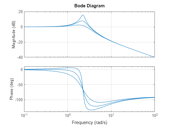
Sensitivity Analysis Example

Using model editing together with LTI array support, you can easily investigate sensitivity to parameter variations. For example, consider the second-order transfer function

$$H(s)=\frac{s+5}{s^2+2\zeta s+5}$$.

You can investigate the effect of the damping parameter zeta on the frequency response by creating three models with different zeta values and comparing their Bode responses:

s = tf('s');

% Create 3 transfer functions with Numerator = s+5 and Denominator = 1
H = repsys(s+5,[1 1 3]);  

% Specify denominators using 3 different zeta values
zeta = [1 .5 .2];
for k = 1:3
  H(:,:,k).Denominator = [1 2*zeta(k) 5];  % zeta(k) -> k-th model
end

% Plot Bode response
bode(H)
grid