Design Requirements
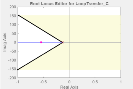
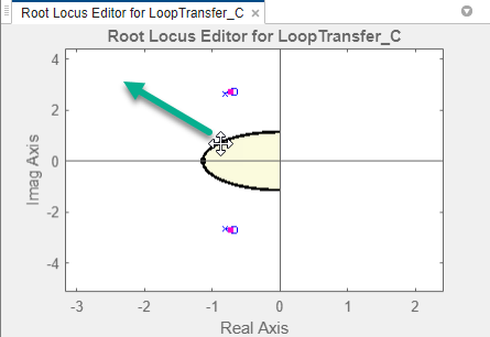
This topic describes time-domain and frequency-domain design requirements available in Control System Designer. Each requirement defines an exclusion region, indicated by a yellow shaded area. To satisfy a requirement, a response plot must remain outside of the associated exclusion region.
If you have Simulink® Design Optimization™ software installed, you can use response optimization techniques to find a compensator that meets your specified design requirements. For examples of optimization-based control design using design requirements, see Optimize LTI System to Meet Frequency-Domain Requirements (Simulink Design Optimization) and Design Optimization-Based PID Controller for Linearized Simulink Model (GUI) (Simulink Design Optimization).
For other Control System Designer tuning methods, you can use the specified design requirements as visual guidelines during the tuning process.
Add Design Requirements
You can add design requirements either directly to existing plots or, when using optimization-based tuning, from the Response Optimization dialog box.
Add Requirements to Existing Plots
You can add design requirements directly to existing:
Bode, root locus, and Nichols editor plots.
Analysis plots:
Root locus plots and pole/zero maps
Bode diagrams
Nichols plots
Step and impulse responses
To add a design requirement to a plot, in Control System Designer, right-click the plot, and select Design Requirements > New.
In the New Design Requirement dialog box, in the Design requirement type drop-down list, select the type of requirement to add. You can select any valid requirement for the associated plot type.
In the Design requirement parameters section, configure the requirement properties. Parameters are dependent on the type of requirement you select.
To create the specified requirement and add it to the plot, click OK.
Add Requirements from Response Optimization Dialog Box
When using optimization-based tuning, you can add design requirements from the Response Optimization dialog box.

To do so, on the Design Requirements tab, click Add New Design Requirement.
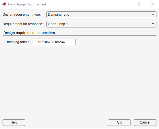
In the New Design Requirement dialog box, select a Design requirement type from the drop-down list.
In the Requirement for response drop-down list, specify the response to which to apply the design requirement. You can select any response in Data Browser.
In the Design requirement parameters section, configure the requirement properties. Parameters are dependent on the type of requirement you select.
To create the specified design requirement, click OK. In the Response Optimization dialog box, on the Design Requirements tab, the new requirement is added to the table.
The app also adds the design requirement to a corresponding editor or analysis plot. The plot type used depends on the selected design requirement type.
If the requirement is for a Bode, root locus, or Nichols plot and:
A corresponding editor plot is open, the requirement is added to that plot.
Only a corresponding analysis plot is open, the requirement is added to that plot.
No corresponding plot is open, the requirement is added to a new Editor plot.
Otherwise, if the requirement is for a different plot type, the requirement is
added to an appropriate analysis plot. For example, a Step requirement
bound is added to a new step analysis plot.
Edit Design Requirements
To edit an existing requirement, in Control System Designer, right-click the corresponding plot, and select Design Requirements > Edit.
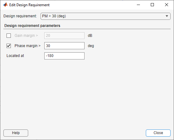
In the Edit Design Requirement dialog box, in the Design requirement drop-down list, select a design requirement to edit. You can select any existing design requirement from the current plot.
In the Design requirement parameters section, specify the requirement properties. Parameters are dependent on the type of requirement you select. When you change a parameter, the app automatically updates the requirement display in the associated plot.
You can also interactively adjust design requirements by dragging the edges or vertices of the shaded exclusion region in the associated plot.
Root Locus and Pole-Zero Plot Requirements
Settling Time
Specifying a settling time for a continuous-time system adds a vertical boundary line to the root locus or pole-zero plot. This line represents pole locations associated with the specified settling time. This boundary is exact for a second-order system with no zeros. For higher order systems, the boundary is an approximation based on second-order dominant systems.
To satisfy this requirement, your system poles must be to the left of the boundary line.
For a discrete-time system, the design requirement boundary is a curved line centered on the origin. In this case, your system poles must be within the boundary line to satisfy the requirement.
Percent Overshoot
Specifying percent overshoot for a continuous-time system adds two rays to the plot that start at the origin. These rays are the locus of poles associated with the specified overshoot value. In the discrete-time case, the design requirement adds two curves originating at (1,0) and meeting on the real axis in the left-hand plane.
Note
The percent overshoot (p.o.) design requirement can be expressed in terms of the damping ratio, ζ:
Damping Ratio
Specifying a damping ratio for a continuous-time system adds two rays to the plot that start at the origin. These rays are the locus of poles associated with the specified overshoot value. This boundary is exact for a second-order system and, for higher order systems, is an approximation based on second-order dominant systems.
To meet this requirement, your system poles must be to the left of the boundary lines.
For discrete-time systems, the design requirement adds two curves originating at (1,0) and meeting on the real axis in the left-hand plane. In this case, your system poles must be within the boundary curves.
Natural Frequency
Specifying a natural frequency bound adds a semicircle to the plot that is centered around the origin. The radius of the semicircle equals the natural frequency.
If you specify a natural frequency lower bound, the system poles must remain outside this semicircle. If you specify a natural frequency upper bound, the system poles must remain within this semicircle.
Region Constraint
To specify a region constraint, define two or more vertices of a piece-wise linear boundary line. For each vertex, specify Real and Imaginary components. This requirement adds a shaded exclusion region on one side of the boundary line. To switch the exclusion region to the opposite side of the boundary, in the response plot, right-click the requirement, and select Flip.
To satisfy this requirement, your system poles must be outside of the exclusion region.
Open-Loop and Closed-Loop Bode Diagram Requirements
Upper Gain Limit
You can specify upper gain limits for both open-loop and closed-loop Bode responses.
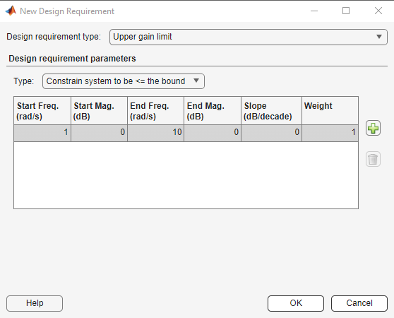
A gain limit consists of one or more line segments. For the start and end points of each segment, specify a frequency, Freq, and magnitude, Mag. You can also specify the slope of the line segment in dB/decade. When you change the slope, the magnitude for the end point updates.
If you are using optimization-based tuning, you can assign a tuning Weight to each segment to indicate their relative importance.
In the Type drop-down list you can select whether to constrain the magnitude to be above or below the specified boundary.
Lower Gain Limit
You can specify lower gain limits in the same way as upper gain limits.
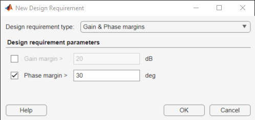
Gain and Phase Margin
You can specify a lower bound for the gain margin, the phase margin, or both. The specified bounds appear in text on the Bode magnitude plot.
Note
Gain and phase margin requirements are only applicable to open-loop Bode diagrams.
Open-Loop Nichols Plot Requirements
Phase Margin
Specify a minimum phase margin as a positive value. Graphically, Control System Designer displays this requirement as a region of exclusion along the 0 dB open-loop gain axis.
Gain Margin
Specify a minimum gain margin value. Graphically, Control System Designer displays this requirement as a region of exclusion along the -180 degree open-loop phase axis.
Closed-Loop Peak Gain
Specify a minimum closed-loop peak gain value. The specified dB value can be positive or negative. The design requirement follows the curves of the Nichols plot grid. As a best practice, have the grid on when using a closed-loop peak gain requirement.
Gain-Phase Design Requirement
To specify a gain-phase design requirement, define two or more vertices of a piece-wise linear boundary line. For each vertex, specify Open-Loop phase and Open-Loop gain values. This requirement adds a shaded exclusion region on one side of the boundary line. To switch the exclusion region to the opposite side of the boundary, in the Nichols plot, right-click the requirement, and select Flip.
Display Location
When editing a phase margin, gain margin, or closed-loop peak gain requirement, you can specify the display location as -180 ± k360 degrees, where k is an integer value.
If you enter an invalid location, the closest valid location is selected. While displayed graphically at only one location, these requirements apply regardless of actual phase; that is, they are applied for all values of k.
Step and Impulse Response Requirements
Upper Time Response Bound
You can specify upper time response bounds for both step and impulse responses.
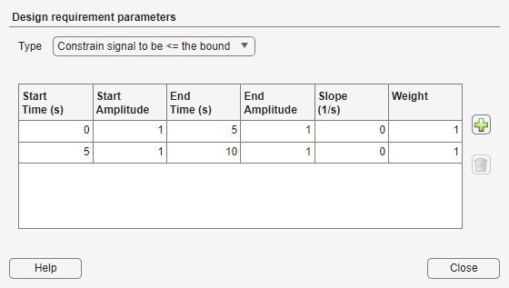
A time-response bound consists of one or more line segments. For the start and end points of each segment, specify a Time and Amplitude value. You can also specify the slope of the line segment. When you change the slope, the amplitude for the end point updates.
If you are using optimization-based tuning, you can assign a tuning Weight to each segment to indicate its relative importance.
In the Type drop-down list, you can select whether to constrain the response to be above or below the specified boundary.
Lower Time Response Bound
You can specify lower time response bounds for both step and impulse responses in the same way as upper gain limits.
Step Response Bound
For a step response plot, you can also specify a step response bound design requirement.
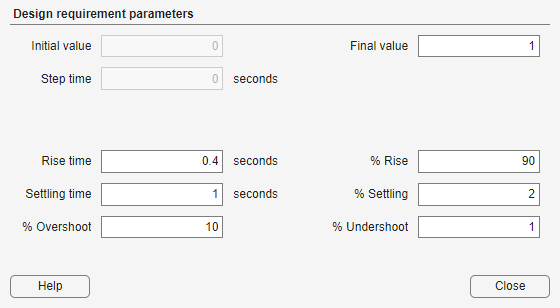
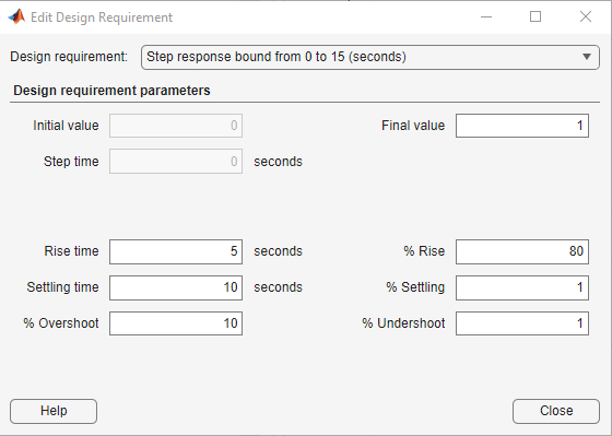
To define a step response bound requirement, specify the following step response parameters:
Final value — Final steady-state value
Rise time — Time required to reach the specified percentage, % Rise, of the Final value
Settling time — Time at which the response enters and stays within the settling percentage, % Settling, of the Final value
% Overshoot — Maximum percentage overshoot above the Final value
% Undershoot — Maximum percentage undershoot below the Initial value
In Control System Designer, step response plots always use an
Initial value and a Step time of
0
See Also
Topics
- Optimize LTI System to Meet Frequency-Domain Requirements (Simulink Design Optimization)
- Design Optimization-Based PID Controller for Linearized Simulink Model (GUI) (Simulink Design Optimization)