Using LTI Arrays for Simulating Multi-Mode Dynamics
This example shows how to construct a Linear Parameter Varying (LPV) representation of a system that exhibits multi-mode dynamics.
Introduction
We often encounter situations where an elastic body collides with, or presses against, a possibly elastic surface. Examples of such situations are:
An elastic ball bouncing on a hard surface.
An engine throttle valve that is constrained to close to no more than
 using a hard spring.
A passenger sitting on a car seat made of polyurethane foam, a viscoelastic material.
In these situations, the motion of the moving body exhibits different dynamics when it is moving freely than when it is in contact with a surface. In the case of a bouncing ball, the motion of the mass can be described by rigid body dynamics when it is falling freely. When the ball collides and deforms while in contact with the surface, the dynamics have to take into account the elastic properties of the ball and of the surface. A simple way of modeling the impact dynamics is to use lumped mass spring-damper descriptions of the colliding bodies. By adjusting the relative stiffness and damping coefficients of the two bodies, we can model the various situations described above.
Modeling Bounce Dynamics
Figure 1 shows a mass-spring-damper model of the system. Mass 1 is falling freely under the influence of gravity. Its elastic properties are described by stiffness constant  and damping coefficient
  . When this mass hits the fixed surface, the impact causes Mass 1 and Mass 2 to move downwards together. After a certain "residence time" during which the Mass 1 deforms and recovers, it loses contact with Mass 2 completely to follow a projectile motion. The overall dynamics are thus broken into two distinct modes - when the masses are not in contact and when they are moving jointly.
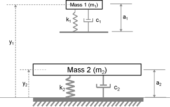
Figure 1: Elastic body bouncing on a fixed elastic surface.
The unstretched (load-free) length of spring attached to Mass 1 is  , while that of Mass 2 is
  . The variables
  and
and  denote the positions of the two masses. When the masses are not in contact ("Mode 1"), their motions are governed by the following equations:


with initial conditions  ,
,  ,
,  ,
,  .
.  is the height from which Mass 1 is originally dropped.
  is the initial location of Mass 2 which corresponds to an unstretched state of its spring.
When Mass 1 touches Mass 2 ("Mode 2"), their displacements and velocities get interlinked. The governing equations in this mode are:


with  , where
  is the time at which Mass 1 first touches Mass 2.
LPV Representation
The governing equations are linear and time invariant. However, there are two distinct behavioral modes corresponding to different equations of motion. Both modes are governed by sets of second order equations. If we pick the positions and velocities of the masses as state variables, we can represent each mode by a 4th order state-space equation.
In the state-space view, it becomes possible to treat the two modes as a single system whose coefficients change as a function of a certain condition which determines which mode is active. The condition is, of course, whether the two masses are moving freely or jointly. Such a representation, where the coefficients of a linear system are parameterized by an external but measurable parameter is called a Linear Parameter Varying (LPV) model. A common representation of an LPV model is by means of an array of linear state-space models and a set of scheduling parameters that dictate the rules for choosing the correct model under a given condition. The array of linear models must all be defined using the same state variables.
For our example, we need two state-space models, one for each mode of operation. We also need to define a scheduling variable to switch between them. We begin by writing the above equations of motion in state-space form.
Define values of masses and their spring constants.
m1 = 7;     % first mass (g)
k1 = 100;   % spring constant for first mass (g/s^2)
c1 = 2;     % damping coefficient associated with first mass (g/s)

m2 = 20;    % second mass (g)
k2 = 300;   % spring constant for second mass (g/s^2)
c2 = 5;     % damping coefficient associated with second mass (g/s)

g = 9.81;   % gravitational acceleration (m/s^2)

a1 = 12;    % uncompressed lengths of spring 1 (mm)
a2 = 20;    % uncompressed lengths of spring 2 (mm)

h1 = 100;   % initial height of mass m1 (mm)
h2 = a2;    % initial height of mass m2 (mm)
First mode: state-space representation of dynamics when the masses are not in contact.
A11 = [0 1; 0 0];
B11 = [0; -g];
C11 = [1 0];
D11 = 0;

A12 = [0 1; -k2/m2, -c2/m2];
B12 = [0; -g+(k2*a2/m2)];
C12 = [1 0];
D12 = 0;

A1 = blkdiag(A11, A12);
B1 = [B11; B12];
C1 = blkdiag(C11, C12);
D1 = [D11; D12];

sys1 = ss(A1,B1,C1,D1);
Second mode: state-space representation of dynamics when the masses are in contact.
A2 = [ 0        1,         0,             0; ...
      -k1/m1,   -c1/m1,    k1/m1,         c1/m1;...
      0,        0,         0,             1; ...
      k1/m2,    c1/m2,     -(k1+k2)/m2,   -(c1+c2)/m2];

B2 = [0; -g+k1*a1/m1; 0; -g+(k2/m2*a2)-(k1/m2*a1)];
C2 = [1 0 0 0; 0 0 1 0];
D2 = [0;0];

sys2 = ss(A2,B2,C2,D2);
Now we stack the two models sys1 and sys2 together to create a state-space array.
sys = stack(1,sys1,sys2);
Use the information on whether the masses are moving freely or jointly for scheduling. Let us call this parameter "FreeMove" which takes the value of 1 when masses are moving freely and 0 when they are in contact and moving jointly. The scheduling parameter information is incorporated into the state-space array object (sys) by using its "SamplingGrid" property:
sys.SamplingGrid = struct('FreeMove',[1; 0]);
Whether the masses are in contact or not is decided by the relative positions of the two masses; when  , the masses are not in contact.
Simulation of LPV Model in Simulink
The state-space array sys has the necessary information to represent an LPV model. You can simulate this model in Simulink® using the LPV System block.
Open the preconfigured Simulink model LPVBouncingMass.slx.
open_system('LPVBouncingMass')
open_system('LPVBouncingMass/Bouncing Mass Model','mask')
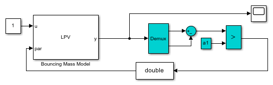
The block called "Bouncing Mass Model" is an LPV System block. Its parameters are specified as follows:
For "State-space array" field, specify the state-space model array
systhat was created above.For "Initial state" field, specify the initial positions and velocities of the two masses. Note that the state vector is:
![$[y_1, \dot{y}_1, y_2, \dot{y}_2]$](../../examples/control/win64/MultiModeSimulationExample_eq11685958539206647682.png) . Specify its value as [h1 0 h2 0]'.
. Specify its value as [h1 0 h2 0]'.Under the "Scheduling" tab, set the "Interpolation method" to "Nearest". This choice causes only one of the two models in the array to be active at any time. In our example, the behavior modes are mutually exclusive.
Under the "Outputs" tab, uncheck all the checkboxes for optional output ports. We will be observing only the positions of the two masses.
The constant block outputs a unit value. This serves as the input to the model and is supplied from the first input port of the LPV block. The block has only one output port which outputs the positions of the two masses as a 2-by-1 vector.
The second input port of the LPV block is for specifying the scheduling signal. As discussed before, this signal represents the scheduling parameter "FreeMove" and takes discrete values 0 (masses in contact) or 1 (masses not in contact). The value of this parameter is computed as a function of the block's output signal. This computation is performed by the blocks with cyan background color. We take the difference between the two outputs (after demuxing) and compare the result to the unstretched length of spring attached to Mass 1. The resulting Boolean result is converted into a double signal which serves as the scheduling parameter value.
We are now ready to perform the simulation.
open_system('LPVBouncingMass/Scope')
sim('LPVBouncingMass')
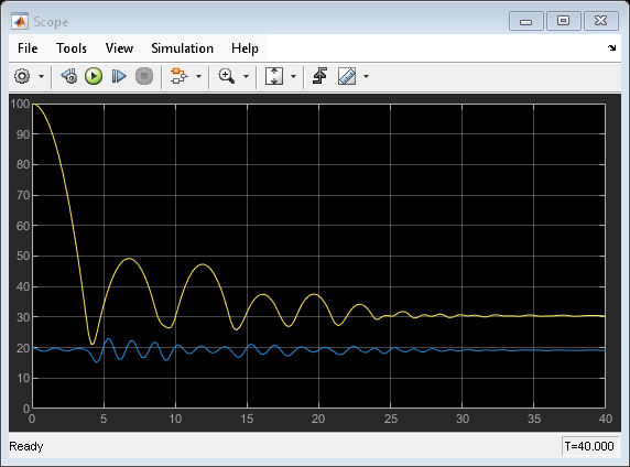
The yellow curve shows the position of Mass 1 while the magenta curve shows the position of Mass 2. At the start of simulation, Mass 1 undergoes free fall until it hits Mass 2. The collision causes the Mass 2 to be displaced but it recoils quickly and bounces Mass 1 back. The two masses are in contact for the time duration where  . When the masses settle down, their equilibrium values are determined by the static settling due to gravity. For example, the absolute location of Mass 1 is
Conclusions
This example shows how a Linear Parameter Varying model can be constructed by using an array of state-space models and suitable scheduling variables. The example describes the case of mutually exclusive modes, although a similar approach can be used in cases where the dynamics behavior at a given value of scheduling parameters is influenced by several linear models.
The LPV System block facilitates the simulation of parameter varying systems. The block also supports code generation for various hardware targets.