Solving a Nonlinear ODE with a Boundary Layer by Collocation

The Problem

We consider the nonlinear singularly perturbed problem

epsilon D^2g(x) + (g(x))^2 = 1 on [0..1]

Dg(0) = g(1) = 0.

This problem is already quite difficult for epsilon = .001, so we choose a modest

epsilon = .1;

The Approximation Space

We seek an approximate solution by collocation from C^1 piecewise cubics with a specified break sequence breaks, hence want the order k to be 4.

breaks = (0:4)/4;
k = 4;

We obtain the corresponding knot sequence as

knots = augknt(breaks,k,2)

knots = 1×14

         0         0         0         0    0.2500    0.2500    0.5000    0.5000    0.7500    0.7500    1.0000    1.0000    1.0000    1.0000

Whatever the choice of order and knots, the corresponding spline space has dimension

n = length(knots) - k

n = 
10

Discretization

The number of degrees of freedom, 10, fits nicely with the fact that we expect to collocate at two sites per polynomial piece, for a total of 8 conditions, bringing us to 10 conditions altogether once we add the two side conditions.

We choose two Gauss sites for each interval. For the `standard' interval [-1/2 .. 1/2] of unit length, these are the two sites

gauss = .5773502692*[-1/2; 1/2];

From this, we obtain the whole collection of collocation sites by

ninterv = length(breaks)-1;
temp = (breaks(2:ninterv+1)+breaks(1:ninterv))/2;
temp = temp([1 1],:) + gauss*diff(breaks);
colsites = temp(:).';

The Numerical Problem

The numerical problem we want to solve is to find a piecewise polynomial (or pp) y of the given order, and with the given knots, that satisfies the nonlinear system

Dy(0) = 0

(y(x))^2 + epsilon D^2y(x) = 1 for x in colsites

y(1) = 0

Linearization

If y is our current approximation to the solution, then the linear problem for the better (?) solution z by Newton's method reads

Dz(0) = 0

w_0(x)z(x) + epsilon D^2z(x) = b(x) for x in colsites

z(1) = 0

with w_0(x) := 2y(x) and b(x) := (y(x))^2 + 1.

In fact, by choosing w_0(1) := 1, w_1(0) := 1, and

w_2(x) := epsilon, w_1(x) := 0 for x in colsites

and choosing all other values of w_0, w_1, w_2, and b not yet specified to be zero, we can give our system the uniform shape

w_0(x)z(x) + w_1(x)Dz(x) + w_2(x)D^2z(x) = b(x) for x in sites

where

sites = [0,colsites,1];

Linear System to be Solved

This system converts into one for the B-spline coefficients of its solution z. For this, we need the zeroth, first, and second derivative at every x in sites and for every relevant B-spline. These values are supplied by the spcol command.

Here is the essential part of the documentation for spcol:

SPCOL B-spline collocation matrix.

COLLOC = SPCOL(KNOTS,K,TAU) is the matrix

[ D^m(i)B_j(TAU(i)) : i=1:length(TAU), j=1:length(KNOTS)-K ],

with D^m(i)B_j the m(i)-fold derivative of B_j,

B_j the j-th B-spline of order K for the knot sequence KNOTS,

TAU a sequence of sites,

both KNOTS and TAU are assumed to be nondecreasing, and

m(i) is the integer #{ j<i : TAU(j) = TAU(i) }, i.e., the

'cumulative' multiplicity of TAU(i) in TAU.

We use spcol to supply the matrix

colmat = spcol(knots,k, brk2knt(sites,3));

with brk2knt used here to triple each entry of sites, and thus we get in colmat, for each x in sites, the value and the first and second derivatives at x of all the relevant B-splines.

From this, we get the collocation matrix by combining the row triple associated with x using the weights w_0(x), w_1(x), w_2(x) to get the row corresponding to x of the matrix of our linear system.

Need Initial Guess for Y

We also need a current approximation y from our spline space. Initially, we get it by interpolating some reasonable initial guess from our pp space at sites. For that guess, we use the parabola

x^2 - 1

which does satisfy the end conditions and lies in our spline space. We obtain its B-form by interpolation at sites. We select the relevant interpolation matrix from the full matrix colmat. Here it is, in several cautious steps:

intmat = colmat([2 1+(1:(n-2))*3,1+(n-1)*3],:);
coefs = intmat\[0 colsites.*colsites-1 0].';
y = spmak(knots,coefs.');

We plot the result, to be sure -- it should be exactly x^2-1.

fnplt(y,'g');
legend('Initial Guess (x^2-1)','location','NW');
axis([-0.01 1.01 -1.01 0.01]);
hold on

Iteration

We can now complete the construction and solution of the linear system for the improved approximate solution z from our current guess y. In fact, with the initial guess y available, we now set up an iteration, to be terminated when the change z-y is less than a specified tolerance.

tolerance = 6.e-9;

The max-norms of the change z-y at each iteration are shown as output below, and the figure shows each of the iterates.

while 1
   vtau = fnval(y,colsites);
   weights = [0 1 0;
            [2*vtau.' zeros(n-2,1) repmat(epsilon,n-2,1)];
            1 0 0];
   colloc = zeros(n,n);
   for j = 1:n
      colloc(j,:) = weights(j,:)*colmat(3*(j-1)+(1:3),:);
   end
   coefs = colloc\[0 vtau.*vtau+1 0].';
   z = spmak(knots,coefs.');
   fnplt(z,'k');
   maxdif = max(max(abs(z.coefs-y.coefs))); 
   fprintf('maxdif = %g\n',maxdif)
   if (maxdif<tolerance), break, end
   
   % now reiterate
   y = z;
end

maxdif = 0.206695
maxdif = 0.01207
maxdif = 3.95151e-05
maxdif = 4.43216e-10

legend({'Initial Guess (x^2-1)' 'Iterates'},'location','NW');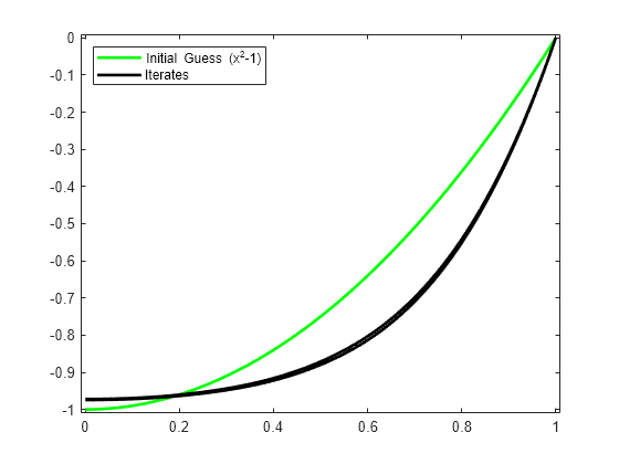

That looks like quadratic convergence, as expected from a Newton iteration.

Getting Ready for a Smaller Epsilon

If we now decrease epsilon, we create more of a boundary layer near the right endpoint, and this calls for a nonuniform mesh. We use newknt to construct an appropriate (finer) mesh from the current approximation.

knots = newknt(z, ninterv+1); 
breaks = knt2brk(knots);
knots = augknt(breaks,4,2);
n = length(knots)-k;

Collocation Sites for New Breaks

Next, we get the collocation sites corresponding to the new breaks

ninterv = length(breaks)-1;
temp = ((breaks(2:ninterv+1)+breaks(1:ninterv))/2);
temp = temp([1 1], :) + gauss*diff(breaks);
colsites = temp(:).';
sites = [0,colsites,1];

and then the new collocation matrix.

colmat = spcol(knots,k, brk2knt(sites,3));

Initial Guess

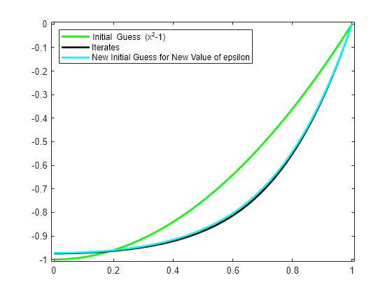
We obtain the initial guess y as the interpolant from the current spline space to the computed solution z. We plot the resulting interpolant to be sure -- it should be close to our current solution.

intmat = colmat([2 1+(1:(n-2))*3,1+(n-1)*3],:);
y = spmak(knots,[0 fnval(z,colsites) 0]/intmat.');
fnplt(y,'c');
ax = gca;
h = ax.Children;
legend(h([6 5 1]),{'Initial Guess (x^2-1)' 'Iterates' ...
                   'New Initial Guess for New Value of epsilon'}, ...
                   'location','NW');

Iteration with Smaller Epsilon

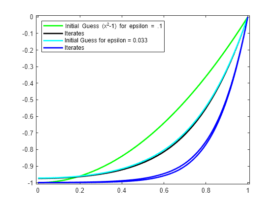
Now we divide epsilon by 3 and repeat the above iteration. Convergence is again quadratic.

epsilon = epsilon/3;
while 1
   vtau = fnval(y,colsites);
   weights = [0 1 0;
            [2*vtau.' zeros(n-2,1) repmat(epsilon,n-2,1)];
            1 0 0];
   colloc = zeros(n,n);
   for j = 1:n
      colloc(j,:) = weights(j,:)*colmat(3*(j-1)+(1:3),:);
   end
   coefs = colloc\[0 vtau.*vtau+1 0].';
   z = spmak(knots,coefs.');
   fnplt(z,'b');
   maxdif = max(max(abs(z.coefs-y.coefs)));
   fprintf('maxdif = %g\n',maxdif)
   if (maxdif<tolerance), break, end
   
   % now reiterate
   y = z;
end

maxdif = 0.237937
maxdif = 0.0184488
maxdif = 0.000120467
maxdif = 4.78116e-09

ax = gca;
h = ax.Children;
legend(h([10 9 5 4]), ...
       {'Initial Guess (x^2-1) for epsilon = .1' 'Iterates' ...
        sprintf('Initial Guess for epsilon = %.3f',epsilon) ...
        'Iterates'}, 'location','NW');

Very Small Epsilon

For a much smaller epsilon, we merely repeat these calculations, dividing epsilon by 3 each time.

for ee = 1:4
   knots = newknt(z, ninterv+1); 
   breaks = knt2brk(knots);
   knots = augknt(breaks,4,2); 
   n = length(knots)-k;

   ninterv = length(breaks)-1;
   temp = ((breaks(2:ninterv+1)+breaks(1:ninterv))/2);
   temp = temp([1 1], :) + gauss*diff(breaks);
   colsites = temp(:).';
   sites = [0,colsites,1];

   colmat = spcol(knots,k, brk2knt(sites,3));

   intmat = colmat([2 1+(1:(n-2))*3,1+(n-1)*3],:);
   y = spmak(knots,[0 fnval(z,colsites) 0]/intmat.');
   fnplt(y,'c')

   epsilon = epsilon/3;
   while 1
      vtau = fnval(y,colsites);
      weights = [0 1 0;
               [2*vtau.' zeros(n-2,1) repmat(epsilon,n-2,1)];
               1 0 0];
      colloc = zeros(n,n);
      for j = 1:n
       colloc(j,:) = weights(j,:)*colmat(3*(j-1)+(1:3),:);
      end
      coefs = colloc\[0 vtau.*vtau+1 0].';
      z = spmak(knots,coefs.');
      fnplt(z,'b');
      maxdif = max(max(abs(z.coefs-y.coefs)));
      if (maxdif<tolerance), break, end
      
      % now reiterate
      y = z;
   end
end
ax = gca;
h = ax.Children;
legend(h([30 29 25 24]), ...
       {'Initial Guess (x^2-1) for epsilon = .1' 'Iterates' ...
        'Initial Guesses for epsilon = .1/3^j, j=1:5' ...
        'Iterates'},'location','NW');

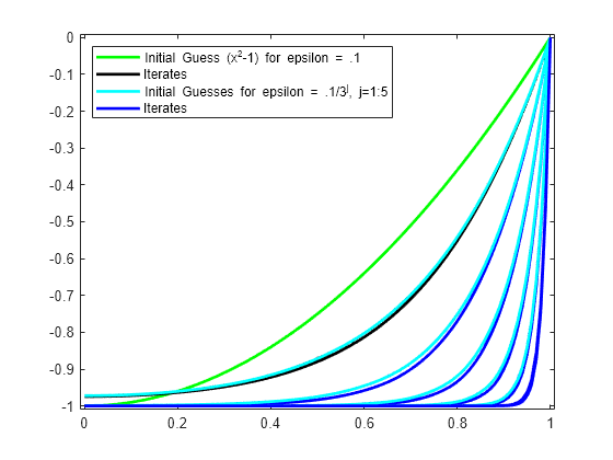
Plot the Breaks Used for Smallest Epsilon

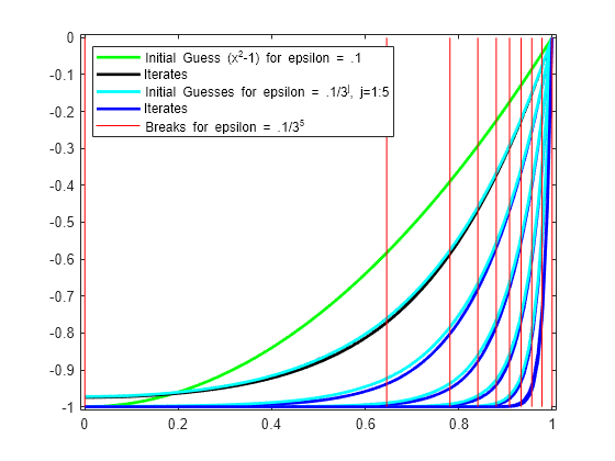
Here is the final distribution of breaks, showing newknt to have worked well in this case.

breaks = fnbrk(fn2fm(z,'pp'),'b');
bb = repmat(breaks,3,1);
cc = repmat([0;-1;NaN],1,length(breaks));
plot(bb(:),cc(:),'r');
hold off
ax = gca;
h = ax.Children;
legend(h([31 30 26 25 1]), ...
       {'Initial Guess (x^2-1) for epsilon = .1' 'Iterates' ...
        'Initial Guesses for epsilon = .1/3^j, j=1:5' ...
        'Iterates' 'Breaks for epsilon = .1/3^5'},'location','NW');

Plot Residual for Smallest Epsilon

Recall that we are solving the ODE

epsilon D^2g(x) + (g(x))^2 = 1 on [0..1]

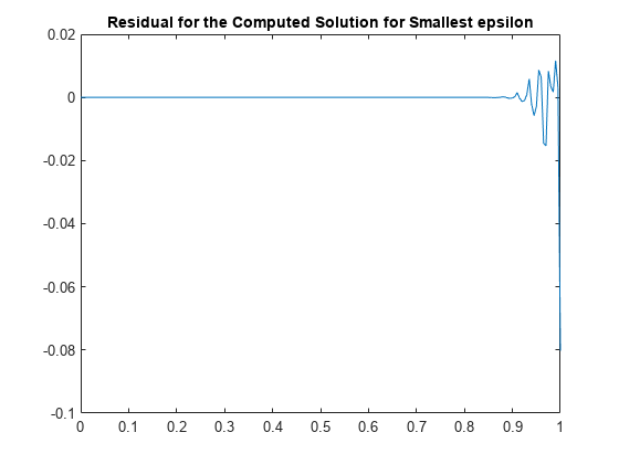
As a check, we compute and plot the residual for the computed solution for the smallest epsilon. This, too, looks satisfactory.

xx = linspace(0,1,201);
plot(xx, 1 - epsilon*fnval(fnder(z,2),xx) - (fnval(z,xx)).^2)
title('Residual for the Computed Solution for Smallest epsilon');