Acquire and Analyze Noisy Clock Signals

Create a DataAcquisition and Acquire a Clock Signal

Use daq to create a DataAcquisition and addinput to add a channel from the National Instruments® NI-9205 with ID of 'cDAQ1Mod1'.

dq = daq("ni");
addinput(dq,"cDAQ1Mod1","ai0","Voltage");

By default the DataAcquisition is configured to run at 1000 scans/second.

Change the scan rate to 250000 scans/second.

dq.Rate = 250000;

Use read to acquire multiple scans for 2 ms.

[data, time] = read(dq, milliseconds(2), "OutputFormat", "Matrix");

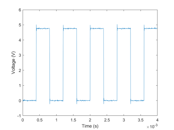
Plot the acquired clock signal (note that it is overdamped).

plot(time, data)
xlabel('Time (s)')
ylabel('Voltage (V)')

Estimate State Levels

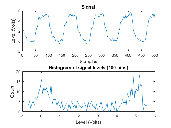
Use statelevels with no output argument to visualize the state levels in a histogram.

statelevels(data)

ans =

    0.0138    5.1848

The computed histogram is divided into two equal sized regions between the first and last bin. The mode of each region of the histogram is returned as an estimated state level value in the command window.

Use optional input arguments to specify the number of histogram bins, histogram bounds, and the state level estimation method.

Measure Rise Time, Fall Time, and Slew Rate

Use risetime with no output argument to visualize the rise time of positive edges.

risetime(data,time)

ans =

   1.0e-04 *

    0.5919
    0.8344
    0.7185
    0.8970
    0.6366

The default reference levels for computing rise time and fall time are set at 10% and 90% of the waveform amplitude.

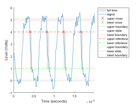
Measure fall time by specifying custom reference and state levels.

falltime(data,time,'PercentReferenceLevels',[20 80],'StateLevels',[0 5])

ans =

   1.0e-04 *

    0.4294
    0.5727
    0.5032
    0.4762

Obtain measurements programmatically by calling functions with one or more output arguments. For uniformly sampled data, you can provide a sample rate in place of the time vector. Use slewrate to measure the slope of each positive or negative edge.

sr = slewrate(data(1:100), dq.Rate)

sr =

   7.0840e+04

Analyze Overshoot and Undershoot

Acquire a new underdamped clock signal.

[data, time] = read(dq, milliseconds(4), "OutputFormat", "Matrix");
plot(time, data)
xlabel('Time (s)')
ylabel('Voltage (V)')

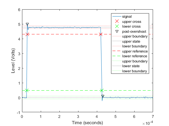
Underdamped clock signals exhibit overshoot. Overshoot is expressed as a percentage of the difference between state levels. Overshoot can occur just after an edge, at the start of the post-transition aberration region. This is called "postshoot" overshoot. Measure the overshoot using overshoot.

overshoot(data(95:270),dq.Rate)
legend('Location','NorthEast')

ans =

    4.9451
    2.5399

Overshoot can also occur just before an edge, at the end of the pre-transition aberration region. This is called "preshoot" overshoot.

Undershoot can occur in the pre-aberration and post-aberration regions and is expressed as a percentage of the difference between the state levels. Measure the undershoot with optional input arguments specifying the region to measure aberrations.

undershoot(data(95:270),dq.Rate,'Region','Postshoot')
legend('Location','NorthEast')

ans =

    3.8499
    4.9451

Measure Pulse Width and Duty Cycle

Use pulsewidth with no output argument to visualize highlighted pulse widths.

pulsewidth(data, time, 'Polarity', 'Positive');

This displays pulses of positive polarity. Select negative polarity to see the widths of negative polarity pulses.

Use dutycycle to compute the ratio of the pulse width to the pulse period for each positive-polarity or negative-polarity pulse. Duty cycles are expressed as a percentage of the pulse period.

d = dutycycle(data,time,'Polarity','negative')

d =

    0.4979
    0.5000
    0.5000

Use pulseperiod to obtain the periods of each cycle of the waveform. Use this information to compute other metrics such as the average frequency of the waveform or the total observed jitter.

pp = pulseperiod(data, time);

avgFreq = 1./mean(pp)
totalJitter = std(pp)

avgFreq =

    1.2500e+03


totalJitter =

   1.9866e-06