Neural Network for Beam Selection
This example shows how to use a neural network to reduce the overhead in the beam selection task. In the example, you use only the location of the receiver rather than knowledge of the communication channels. Instead of an exhaustive beam search over all the beam pairs, you can reduce beam sweeping overhead by searching among the selected beam pairs. Considering a system with a total of 16 beam pairs, simulation results in this example show the designed machine learning algorithm can achieve an accuracy of 90% by performing an exhaustive search over only half of the beam pairs.
Introduction
To enable millimeter wave (mmWave) communications, beam management techniques must be used due to the high pathloss and blockage experienced at high frequencies. Beam management is a set of Layer 1 (physical layer) and Layer 2 (medium access control) procedures to establish and retain an optimal beam pair (transmit beam and a corresponding receive beam) for good connectivity [1]. For simulations of 5G New Radio (NR) beam management procedures, see the NR SSB Beam Sweeping (5G Toolbox) and NR Downlink Transmit-End Beam Refinement Using CSI-RS (5G Toolbox) examples.
This example considers beam selection procedures when a connection is established between the user equipment (UE) and access network node (gNB). In 5G NR, the beam selection procedure for initial access consists of beam sweeping, which requires exhaustive searches over all the beams on the transmitter and the receiver sides, and then selection of the beam pair offering the strongest reference signal received power (RSRP). Since mmWave communications require many antenna elements, implying many beams, an exhaustive search over all beams becomes computationally expensive and increases the initial access time.
To avoid repeatedly performing an exhaustive search and to reduce the communication overhead, machine learning has been applied to the beam selection problem. Typically, the beam selection problem is posed as a classification task, where the target output is the best beam pair index. The extrinsic information, including lidar, GPS signals, and roadside camera images, is used as input to the machine learning algorithms [2]-[6]. Specifically, given this out-of-band information, a trained machine learning model recommends a set of good beam pairs. Instead of an exhaustive search over all the beam pairs, the simulation reduces beam sweeping overhead by searching only among the selected beam pairs.
This example uses a neural network to perform beam selection using only the GPS coordinates of the receiver. Fixing the locations of the transmitter and the scatterers, the example generates a set of training samples: Each sample consists of a receiver location (GPS data) and the true optimal beam pair index (found by performing exhaustive search over all the beam pairs at transmit and receive ends). The example designs and trains a neural network that uses the location of the receiver as the input and the true optimal beam pair index as the correct label. During the testing phase, the neural network first outputs good beam pairs. An exhaustive search over these beam pairs is followed, and the beam pair with the highest average RSRP is selected as the final predicted beam pair by the neural network.
The example measures the effectiveness of the proposed method using two metrics: average RSRP and top-K accuracy [2]-[6]. This figure shows the main processing steps.

rng(211); % Set RNG state for repeatabilityGenerate Training Data
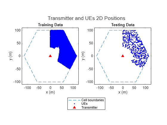
In the prerecorded data, receivers are randomly distributed on the perimeter of a 6-meter square and configured with 16 beam pairs (four beams on each end, analog beamformed with 1 RF chain). After setting up a MIMO scattering channel, the example considers 200 different receiver locations in the training set and 100 different receiver locations in the test sets. The prerecorded data uses 2-D location coordinates. Specifically, the third GPS coordinate of each sample is always zero. As in the NR SSB Beam Sweeping example, for each location, SSB-based beam sweeping is performed for an exhaustive search over all 16 beam pairs. Since AWGN is added during the exhaustive search, for each location, the example runs four different trials and determines the true optimal beam pair by picking the beam pair with the highest average RSRP.
To generate new training and test sets, you can adjust the useSavedData and SaveData logicals. Be aware that regenerating data takes a significant amount of time.
useSavedData = true;
saveData = false;

if useSavedData
    load nnBS_prm.mat;              % Load beam selection system parameters
    load nnBS_TrainingData.mat;     % Load prerecorded training samples
    %   (input: receiver's location; output: optimal beam pair indices)
    load nnBS_TestData.mat;         % Load prerecorded test samples
else
Configure Frequency and Beam Sweeping Angles
    prm.NCellID = 1;                    % Cell ID
    prm.FreqRange = 'FR1';              % Frequency range: 'FR1' or 'FR2'

    prm.CenterFreq = 2.5e9;             % Hz
    prm.SSBlockPattern = 'Case B';      % Case A/B/C/D/E
    prm.SSBTransmitted = [ones(1,4) zeros(1,0)]; % 4/8 or 64 in length

    prm.TxArraySize = [8 8];            % Transmit array size, [rows cols]
    prm.TxAZlim = [-163 177];           % Transmit azimuthal sweep limits
    prm.TxELlim = [-90 0];              % Transmit elevation sweep limits

    prm.RxArraySize = [2 2];            % Receive array size, [rows cols]
    prm.RxAZlim = [-177 157];           % Receive azimuthal sweep limits
    prm.RxELlim = [0 90];               % Receive elevation sweep limits

    prm.ElevationSweep = false;         % Enable/disable elevation sweep
    prm.SNRdB = 30;                     % SNR, dB
    prm.RSRPMode = 'SSSwDMRS';          % {'SSSwDMRS', 'SSSonly'}

    prm = validateParams(prm);
Synchronization Signal Burst Configuration
    txBurst = nrWavegenSSBurstConfig;
    txBurst.BlockPattern = prm.SSBlockPattern;
    txBurst.TransmittedBlocks = prm.SSBTransmitted;
    txBurst.Period = 20;
    txBurst.SubcarrierSpacingCommon = prm.SubcarrierSpacingCommon;
Scatterer Configuration
    c = physconst('LightSpeed');   % Propagation speed
    prm.lambda = c/prm.CenterFreq; % Wavelength

    prm.rightCoorMax = 10;    % Maximum x-coordinate
    prm.topCoorMax = 10;      % Maximum y-coordinate
    prm.posTx = [3.5;4.2;0];  % Transmit array position, [x;y;z], meters

    % Scatterer locations
    % Generate scatterers at random positions
    Nscat = 10;        % Number of scatterers
    azRange = prm.TxAZlim(1):prm.TxAZlim(2);
    elRange = -90:90;

    % More evenly spaced scatterers
    randAzOrder = round(linspace(1, length(azRange), Nscat));
    azAngInSph = azRange(randAzOrder(1:Nscat));

    % Consider a 2-D area, i.e., the elevation angle is zero
    elAngInSph = zeros(size(azAngInSph));
    r = 2;            % radius
    [x,y,z] = sph2cart(deg2rad(azAngInSph),deg2rad(elAngInSph),r);
    prm.ScatPos = [x;y;z] + [prm.rightCoorMax/2;prm.topCoorMax/2;0];
Antenna Array Configuration
    % Transmit array
    if prm.IsTxURA
        % Uniform rectangular array
        arrayTx = phased.URA(prm.TxArraySize,0.5*prm.lambda, ...
            'Element',phased.IsotropicAntennaElement('BackBaffled',true));
    else
        % Uniform linear array
        arrayTx = phased.ULA(prm.NumTx, ...
            'ElementSpacing',0.5*prm.lambda, ...
            'Element',phased.IsotropicAntennaElement('BackBaffled',true));
    end

    % Receive array
    if prm.IsRxURA
        % Uniform rectangular array
        arrayRx = phased.URA(prm.RxArraySize,0.5*prm.lambda, ...
            'Element',phased.IsotropicAntennaElement);
    else
        % Uniform linear array
        arrayRx = phased.ULA(prm.NumRx, ...
            'ElementSpacing',0.5*prm.lambda, ...
            'Element',phased.IsotropicAntennaElement);
    end
Determine Tx/Rx Positions
    % Receiver locations
    % Training data: X points around a rectangle: each side has X/4 random points
    % X: X/4 for around square, X/10 for validation => lcm(4,10) = 20 smallest
    NDiffLocTrain = 200;
    pointsEachSideTrain = NDiffLocTrain/4;
    prm.NDiffLocTrain = NDiffLocTrain;

    locationX = 2*ones(pointsEachSideTrain, 1);
    locationY = 2 + (8-2)*rand(pointsEachSideTrain, 1);

    locationX = [locationX; 2 + (8-2)*rand(pointsEachSideTrain, 1)];
    locationY = [locationY; 8*ones(pointsEachSideTrain, 1)];

    locationX = [locationX; 8*ones(pointsEachSideTrain, 1)];
    locationY = [locationY; 2 + (8-2)*rand(pointsEachSideTrain, 1)];

    locationX = [locationX; 2 + (8-2)*rand(pointsEachSideTrain, 1)];
    locationY = [locationY; 2*ones(pointsEachSideTrain, 1)];

    locationZ = zeros(size(locationX));
    locationMat = [locationX locationY locationZ];

    % Fixing receiver's location, run repeated simulations to consider
    % different realizations of AWGN
    prm.NRepeatSameLoc = 4;

    locationMatTrain = repelem(locationMat,prm.NRepeatSameLoc, 1);

    % Test data: Y points around a rectangle: each side has Y/4 random points
    % Different data than test, but a smaller number
    NDiffLocTest = 100;
    pointsEachSideTest = NDiffLocTest/4;
    prm.NDiffLocTest = NDiffLocTest;

    locationX = 2*ones(pointsEachSideTest, 1);
    locationY = 2 + (8-2)*rand(pointsEachSideTest, 1);

    locationX = [locationX; 2 + (8-2)*rand(pointsEachSideTest, 1)];
    locationY = [locationY; 8*ones(pointsEachSideTest, 1)];

    locationX = [locationX; 8*ones(pointsEachSideTest, 1)];
    locationY = [locationY; 2 + (8-2)*rand(pointsEachSideTest, 1)];

    locationX = [locationX; 2 + (8-2)*rand(pointsEachSideTest, 1)];
    locationY = [locationY; 2*ones(pointsEachSideTest, 1)];

    locationZ = zeros(size(locationX));
    locationMat = [locationX locationY locationZ];

    locationMatTest = repelem(locationMat,prm.NRepeatSameLoc,1);

    [optBeamPairIdxMatTrain,rsrpMatTrain] = hGenDataMIMOScatterChan('training',locationMatTrain,prm,txBurst,arrayTx,arrayRx,311);
    [optBeamPairIdxMatTest,rsrpMatTest] = hGenDataMIMOScatterChan('test',locationMatTest,prm,txBurst,arrayTx,arrayRx,411);

    % Save generated data
    if saveData
        save('nnBS_prm.mat','prm');
        save('nnBS_TrainingData.mat','optBeamPairIdxMatTrain','rsrpMatTrain','locationMatTrain');
        save('nnBS_TestData.mat','optBeamPairIdxMatTest','rsrpMatTest','locationMatTest');
    end
end
Plot Transmitter and Scatterer Locations
figure
scatter(prm.posTx(1),prm.posTx(2),100,'r^','filled');
hold on;
scatter(prm.ScatPos(1,:),prm.ScatPos(2,:),100,[0.9290 0.6940 0.1250],'s','filled');
xlim([0 10])
ylim([0 10])
title('Transmitter and Scatterers Positions')
legend('Transmitter','Scatterers')
xlabel('x (m)')
ylabel('y (m)')
Data Processing and Visualization
Next, label the beam pair with the highest average RSRP as the true optimal beam pair. Convert one-hot encoding labels to categorical data to use for classification. Finally, augment the categorical data so that it has 16 classes total to match the possible number of beam pairs (although classes may have unequal number of elements). The augmentation is to ensure that the output of the neural network has the desired dimension 16.
Process Training Data
% Choose the best beam pair by picking the one with the highest average RSRP
% (taking average over NRepeatSameLoc different trials at each location)
avgOptBeamPairIdxCellTrain = cell(size(optBeamPairIdxMatTrain, 1)/prm.NRepeatSameLoc, 1);
avgOptBeamPairIdxScalarTrain = zeros(size(optBeamPairIdxMatTrain, 1)/prm.NRepeatSameLoc, 1);
for locIdx = 1:size(optBeamPairIdxMatTrain, 1)/prm.NRepeatSameLoc
    avgRsrp = squeeze(rsrpMatTrain(:,:,locIdx));
    [~, targetBeamIdx] = max(avgRsrp(:));
    avgOptBeamPairIdxScalarTrain(locIdx) = targetBeamIdx;
    avgOptBeamPairIdxCellTrain{locIdx} = num2str(targetBeamIdx);
end

% Even though there are a total of 16 beam pairs, due to the fixed topology
% (transmitter/scatterers/receiver locations), it is possible
% that some beam pairs are never selected as an optimal beam pair
%
% Therefore, we augment the categories so 16 classes total are in the data
% (although some classes may have zero elements)
allBeamPairIdxCell = cellstr(string((1:prm.numBeams^2)'));
avgOptBeamPairIdxCellTrain = categorical(avgOptBeamPairIdxCellTrain, allBeamPairIdxCell);
NBeamPairInTrainData = numel(categories(avgOptBeamPairIdxCellTrain)); % Should be 16
Process Testing Data
% Decide the best beam pair by picking the one with the highest avg. RSRP
avgOptBeamPairIdxCellTest = cell(size(optBeamPairIdxMatTest, 1)/prm.NRepeatSameLoc, 1);
avgOptBeamPairIdxScalarTest = zeros(size(optBeamPairIdxMatTest, 1)/prm.NRepeatSameLoc, 1);
for locIdx = 1:size(optBeamPairIdxMatTest, 1)/prm.NRepeatSameLoc
    avgRsrp = squeeze(rsrpMatTest(:,:,locIdx));
    [~, targetBeamIdx] = max(avgRsrp(:));
    avgOptBeamPairIdxScalarTest(locIdx) = targetBeamIdx;
    avgOptBeamPairIdxCellTest{locIdx} = num2str(targetBeamIdx);
end
% Augment the categories such that the data has 16 classes total
avgOptBeamPairIdxCellTest = categorical(avgOptBeamPairIdxCellTest, allBeamPairIdxCell);
NBeamPairInTestData = numel(categories(avgOptBeamPairIdxCellTest)); % Should be 16
Create Input/Output Data for Neural Network
trainDataLen = size(locationMatTrain, 1)/prm.NRepeatSameLoc;
trainOut = avgOptBeamPairIdxCellTrain;
sampledLocMatTrain = locationMatTrain(1:prm.NRepeatSameLoc:end, :);
trainInput = sampledLocMatTrain(1:trainDataLen, :);

% Take 10% data out of test data as validation data
valTestDataLen = size(locationMatTest, 1)/prm.NRepeatSameLoc;
valDataLen = round(0.1*size(locationMatTest, 1))/prm.NRepeatSameLoc;
testDataLen = valTestDataLen-valDataLen;

% Randomly shuffle the test data such that the distribution of the
% extracted validation data is closer to test data
rng(111)
shuffledIdx = randperm(prm.NDiffLocTest);
avgOptBeamPairIdxCellTest = avgOptBeamPairIdxCellTest(shuffledIdx);
avgOptBeamPairIdxScalarTest = avgOptBeamPairIdxScalarTest(shuffledIdx);
rsrpMatTest = rsrpMatTest(:,:,shuffledIdx);

valOut = avgOptBeamPairIdxCellTest(1:valDataLen, :);
testOutCat = avgOptBeamPairIdxCellTest(1+valDataLen:end, :);

sampledLocMatTest = locationMatTest(1:prm.NRepeatSameLoc:end, :);
sampledLocMatTest = sampledLocMatTest(shuffledIdx, :);

valInput = sampledLocMatTest(1:valDataLen, :);
testInput = sampledLocMatTest(valDataLen+1:end, :);
Plot Optimal Beam Pair Distribution for Training Data
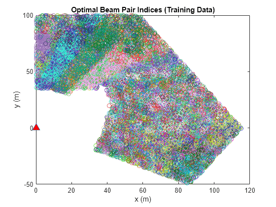
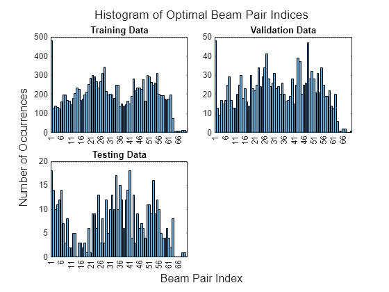
Plot the location and the optimal beam pair for each training sample (200 in total). Each color represents one beam pair index. In other words, the data points with the same color belong to the same class. Increase the training data set to possibly include each beam pair value, though the actual distribution of the beam pairs would depend on the scatterer and transmitter locations.
figure
rng(111)    % for colors in plot
color = rand(NBeamPairInTrainData, 3);
uniqueOptBeamPairIdx = unique(avgOptBeamPairIdxScalarTrain);
for n = 1:length(uniqueOptBeamPairIdx)
    beamPairIdx = find(avgOptBeamPairIdxScalarTrain == uniqueOptBeamPairIdx(n));
    locX = sampledLocMatTrain(beamPairIdx, 1);
    locY = sampledLocMatTrain(beamPairIdx, 2);
    scatter(locX, locY, [], color(n, :));
    hold on;
end
scatter(prm.posTx(1),prm.posTx(2),100,'r^','filled');
scatter(prm.ScatPos(1,:),prm.ScatPos(2,:),100,[0.9290 0.6940 0.1250],'s','filled');
hold off
xlabel('x (m)')
ylabel('y (m)')
xlim([0 10])
ylim([0 10])
title('Optimal Beam Pair Indices (Training Data)')
figure
histogram(trainOut)
title('Histogram of Optimal Beam Pair Indices (Training Data)')
xlabel('Beam Pair Index')
ylabel('Number of Occurrences')
Plot Optimal Beam Pair Distribution for Validation Data
figure
rng(111)    % for colors in plot
color = rand(NBeamPairInTestData, 3);
uniqueOptBeamPairIdx = unique(avgOptBeamPairIdxScalarTest(1:valDataLen));
for n = 1:length(uniqueOptBeamPairIdx)
    beamPairIdx = find(avgOptBeamPairIdxScalarTest(1:valDataLen) == uniqueOptBeamPairIdx(n));
    locX = sampledLocMatTest(beamPairIdx, 1);
    locY = sampledLocMatTest(beamPairIdx, 2);
    scatter(locX, locY, [], color(n, :));
    hold on;
end
scatter(prm.posTx(1),prm.posTx(2),100,'r^','filled');
scatter(prm.ScatPos(1,:),prm.ScatPos(2,:),100,[0.9290 0.6940 0.1250],'s','filled');
hold off
xlabel('x (m)')
ylabel('y (m)')
xlim([0 10])
ylim([0 10])
title('Optimal Beam Pair Indices (Validation Data)')

figure
histogram(valOut)
title('Histogram of Optimal Beam Pair Indices (Validation Data)')
xlabel('Beam Pair Index')
ylabel('Number of Occurrences')
Plot Optimal Beam Pair Distribution for Test Data
figure
rng(111)    % for colors in plots
color = rand(NBeamPairInTestData, 3);
uniqueOptBeamPairIdx = unique(avgOptBeamPairIdxScalarTest(1+valDataLen:end));
for n = 1:length(uniqueOptBeamPairIdx)
    beamPairIdx = find(avgOptBeamPairIdxScalarTest(1+valDataLen:end) == uniqueOptBeamPairIdx(n));
    locX = sampledLocMatTest(beamPairIdx, 1);
    locY = sampledLocMatTest(beamPairIdx, 2);
    scatter(locX, locY, [], color(n, :));
    hold on;
end
scatter(prm.posTx(1),prm.posTx(2),100,'r^','filled');
scatter(prm.ScatPos(1,:),prm.ScatPos(2,:),100,[0.9290 0.6940 0.1250],'s','filled');
hold off
xlabel('x (m)')
ylabel('y (m)')
xlim([0 10])
ylim([0 10])
title('Optimal Beam Pair Indices (Test Data)')
figure
histogram(testOutCat)
title('Histogram of Optimal Beam Pair Indices (Test Data)')
xlabel('Beam Pair Index')
ylabel('Number of Occurrences')

Design and Train Neural Network
Train a neural network with four hidden layers. The design is motivated by [3] (four hidden layers) and [5] (two hidden layers with 128 neurons in each layer) in which the receiver locations are also considered as the input to the neural network. To enable training, adjust the doTraining logical.
This example also provides an option to weight the classes. Classes that occur more frequently have smaller weights and classes that occur less frequently have larger weights. To use class weighting, adjust the useDiffClassWeights logical.
Modify the network to experiment with different designs. If you modify one of the provided data sets, you must retrain the network with the modified data sets. Retraining the network can take a significant amount of time. Adjust the saveNet logical to use the trained network in subsequent runs.
doTraining =false; useDiffClassWeights =
false; saveNet =
false; if doTraining if useDiffClassWeights catCount = countcats(trainOut); %#ok<UNRCH> catFreq = catCount/length(trainOut); nnzIdx = (catFreq ~= 0); medianCount = median(catFreq(nnzIdx)); classWeights = 10*ones(size(catFreq)); classWeights(nnzIdx) = medianCount./catFreq(nnzIdx); filename = 'nnBS_trainedNetwWeighting.mat'; else classWeights = ones(1,NBeamPairInTestData); filename = 'nnBS_trainedNet.mat'; end % Neural network design layers = [ ... featureInputLayer(3,'Name','input','Normalization','rescale-zero-one') fullyConnectedLayer(96,'Name','linear1') leakyReluLayer(0.01,'Name','leakyRelu1') fullyConnectedLayer(96,'Name','linear2') leakyReluLayer(0.01,'Name','leakyRelu2') fullyConnectedLayer(96,'Name','linear3') leakyReluLayer(0.01,'Name','leakyRelu3') fullyConnectedLayer(96,'Name','linear4') leakyReluLayer(0.01,'Name','leakyRelu4') fullyConnectedLayer(NBeamPairInTrainData,'Name','linear5') softmaxLayer('Name','softmax')]; maxEpochs = 1000; miniBatchSize = 256; options = trainingOptions('adam', ... 'MaxEpochs',maxEpochs, ... 'MiniBatchSize',miniBatchSize, ... 'InitialLearnRate',1e-4, ... 'ValidationData',{valInput,valOut}, ... 'ValidationFrequency',500, ... 'OutputNetwork', 'best-validation-loss', ... 'Shuffle','every-epoch', ... 'Plots','none', ... 'ExecutionEnvironment','cpu', ... 'Verbose',true); % Train the network net = trainnet(trainInput,trainOut,layers,@(x,t) crossentropy(x,t,classWeights,WeightsFormat='C'),options); if saveNet save(filename,'net'); end else if useDiffClassWeights load 'nnBS_trainedNetwWeighting.mat'; else load 'nnBS_trainedNet.mat'; end end
Compare Different Approaches: Top-K Accuracy
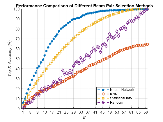
This section tests the trained network with unseen test data considering the top-K accuracy metric. The top-K accuracy metric has been widely used in the neural network-based beam selection task [2]-[6].
Given a receiver location, the neural network first outputs recommended beam pairs. Then it performs an exhaustive sequential search on these beam pairs and selects the one with the highest average RSRP as the final prediction. If the true optimal beam pair is the final selected beam pair, then a successful prediction occurs. Equivalently, a success occurs when the true optimal beam pair is one of the recommended beam pairs by the neural network.
Three benchmarks are compared. Each scheme produces the recommended beam pairs.
KNN - For a test sample, this method first collects closest training samples based on GPS coordinates. The method then recommends all the beam pairs associated with these training samples. Since each training sample has a corresponding optimal beam pair, the number of beam pairs recommended is at most (some beam pairs might be the same).
Statistical Info [5] - This method first ranks all the beam pairs according to their relative frequency in the training set, and then always selects the first beam pairs.
Random [5] - For a test sample, this method randomly chooses beam pairs.
The plot shows that for , the accuracy is already more than 90%, which highlights the effectiveness of using the trained neural network for the beam selection task. When , every scheme (except KNN) is relaxed to the exhaustive search over all the 16 beam pairs, and hence achieves an accuracy of 100%. However, when KNN considers 16 closest training samples, and the number of distinct beam pairs from these samples is often less than 16. Hence, KNN does not achieve an accuracy of 100%.
rng(111)    % for repeatability of the "Random" policy
testOut = avgOptBeamPairIdxScalarTest(1+valDataLen:end, :);
statisticCount = countcats(testOutCat);
predTestOutput = predict(net,testInput);

K = prm.numBeams^2;
accNeural = zeros(1,K);
accKNN = zeros(1,K);
accStatistic = zeros(1,K);
accRandom = zeros(1,K);
for k = 1:K
    predCorrectNeural = zeros(testDataLen,1);
    predCorrectKNN = zeros(testDataLen,1);
    predCorrectStats = zeros(testDataLen,1);
    predCorrectRandom = zeros(testDataLen,1);
    knnIdx = knnsearch(trainInput,testInput,'K',k);

    for n = 1:testDataLen
        trueOptBeamIdx = testOut(n);

        % Neural Network
        [~, topKPredOptBeamIdx] = maxk(predTestOutput(n, :),k);
        if sum(topKPredOptBeamIdx == trueOptBeamIdx) > 0
            % if true, then the true correct index belongs to one of the K predicted indices
            predCorrectNeural(n,1) = 1;
        end

        % KNN
        neighborsIdxInTrainData = knnIdx(n,:);
        topKPredOptBeamIdx= avgOptBeamPairIdxScalarTrain(neighborsIdxInTrainData);
        if sum(topKPredOptBeamIdx == trueOptBeamIdx) > 0
            % if true, then the true correct index belongs to one of the K predicted indices
            predCorrectKNN(n,1) = 1;
        end

        % Statistical Info
        [~, topKPredOptBeamIdx] = maxk(statisticCount,k);
        if sum(topKPredOptBeamIdx == trueOptBeamIdx) > 0
            % if true, then the true correct index belongs to one of the K predicted indices
            predCorrectStats(n,1) = 1;
        end

        % Random
        topKPredOptBeamIdx = randperm(prm.numBeams*prm.numBeams,k);
        if sum(topKPredOptBeamIdx == trueOptBeamIdx) > 0
            % if true, then the true correct index belongs to one of the K predicted indices
            predCorrectRandom(n,1) = 1;
        end

    end

    accNeural(k)    = sum(predCorrectNeural)/testDataLen*100;
    accKNN(k)       = sum(predCorrectKNN)/testDataLen*100;
    accStatistic(k) = sum(predCorrectStats)/testDataLen*100;
    accRandom(k)    = sum(predCorrectRandom)/testDataLen*100;

end

figure
lineWidth = 1.5;
colorNeural = [0 0.4470 0.7410];
colorKNN = [0.8500 0.3250 0.0980];
colorStats = [0.4940 0.1840 0.5560];
colorRandom = [0.4660 0.6740 0.1880];
plot(1:K,accNeural,'--*','LineWidth',lineWidth,'Color',colorNeural)
hold on
plot(1:K,accKNN,'--o','LineWidth',lineWidth,'Color',colorKNN)
plot(1:K,accStatistic,'--s','LineWidth',lineWidth,'Color',colorStats)
plot(1:K,accRandom,'--d','LineWidth',lineWidth,'Color',colorRandom)
hold off
grid on
xticks(1:K)
xlabel('$K$','interpreter','latex')
ylabel('Top-$K$ Accuracy','interpreter','latex')
title('Performance Comparison of Different Beam Pair Selection Schemes')
legend('Neural Network','KNN','Statistical Info','Random','Location','best')

Compare Different Approaches: Average RSRP
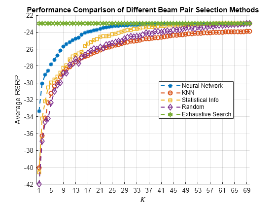
Using unseen test data, compute the average RSRP achieved by the neural network and the three benchmarks. The plot shows that using the trained neural network results in an average RSRP close to the optimal exhaustive search.
rng(111)    % for repeatability of the "Random" policy
K = prm.numBeams^2;
rsrpOptimal = zeros(1,K);
rsrpNeural = zeros(1,K);
rsrpKNN = zeros(1,K);
rsrpStatistic = zeros(1,K);
rsrpRandom = zeros(1,K);
for k = 1:K
    rsrpSumOpt = 0;
    rsrpSumNeural = 0;
    rsrpSumKNN = 0;
    rsrpSumStatistic = 0;
    rsrpSumRandom = 0;

    knnIdx = knnsearch(trainInput,testInput,'K',k);

    for n = 1:testDataLen
        % Exhaustive Search
        trueOptBeamIdx = testOut(n);
        rsrp = rsrpMatTest(:,:,valDataLen+n);
        rsrpSumOpt = rsrpSumOpt + rsrp(trueOptBeamIdx);

        % Neural Network
        [~, topKPredOptCatIdx] = maxk(predTestOutput(n, :),k);
        rsrpSumNeural = rsrpSumNeural + max(rsrp(topKPredOptCatIdx));

        % KNN
        neighborsIdxInTrainData = knnIdx(n,:);
        topKPredOptBeamIdxKNN = avgOptBeamPairIdxScalarTrain(neighborsIdxInTrainData);
        rsrpSumKNN = rsrpSumKNN + max(rsrp(topKPredOptBeamIdxKNN));

        % Statistical Info
        [~, topKPredOptCatIdxStat] = maxk(statisticCount,k);
        rsrpSumStatistic = rsrpSumStatistic + max(rsrp(topKPredOptCatIdxStat));

        % Random
        topKPredOptBeamIdxRand = randperm(prm.numBeams*prm.numBeams,k);
        rsrpSumRandom = rsrpSumRandom + max(rsrp(topKPredOptBeamIdxRand));
    end
    rsrpOptimal(k)  = rsrpSumOpt/testDataLen/prm.NRepeatSameLoc;
    rsrpNeural(k)   = rsrpSumNeural/testDataLen/prm.NRepeatSameLoc;
    rsrpKNN(k)      = rsrpSumKNN/testDataLen/prm.NRepeatSameLoc;
    rsrpStatistic(k) = rsrpSumStatistic/testDataLen/prm.NRepeatSameLoc;
    rsrpRandom(k)   = rsrpSumRandom/testDataLen/prm.NRepeatSameLoc;
end

figure
lineWidth = 1.5;
plot(1:K,rsrpOptimal,'--h','LineWidth',lineWidth,'Color',[0.6350 0.0780 0.1840]);
hold on
plot(1:K,rsrpNeural,'--*','LineWidth',lineWidth,'Color',colorNeural)
plot(1:K,rsrpKNN,'--o','LineWidth',lineWidth,'Color',colorKNN)
plot(1:K,rsrpStatistic,'--s','LineWidth',lineWidth,'Color',colorStats)
plot(1:K,rsrpRandom,'--d','LineWidth',lineWidth, 'Color',colorRandom)
hold off
grid on
xticks(1:K)
xlabel('$K$','interpreter','latex')
ylabel('Average RSRP')
title('Performance Comparison of Different Beam Pair Selection Schemes')
legend('Exhaustive Search','Neural Network','KNN','Statistical Info','Random','Location','best')

Compare the end values for the optimal, neural network, and KNN approaches.
[rsrpOptimal(end-3:end); rsrpNeural(end-3:end); rsrpKNN(end-3:end);]
ans = 3×4

   80.7363   80.7363   80.7363   80.7363
   80.7363   80.7363   80.7363   80.7363
   80.5067   80.5068   80.5069   80.5212
The performance gap between KNN and the optimal methods indicates that the KNN might not perform well even when a larger set of beam pairs is considered, say, 256.
Plot Confusion Matrix
We observe that the classes with fewer elements are negatively impacted with the trained network. Using different weights for different classes could avoid this. Explore the same with the useDiffClassWeights logical and specify custom weights per class.
scores = predict(net,testInput);
predLabels = scores2label(scores,allBeamPairIdxCell);
figure;
cm = confusionchart(testOutCat,predLabels);
title('Confusion Matrix')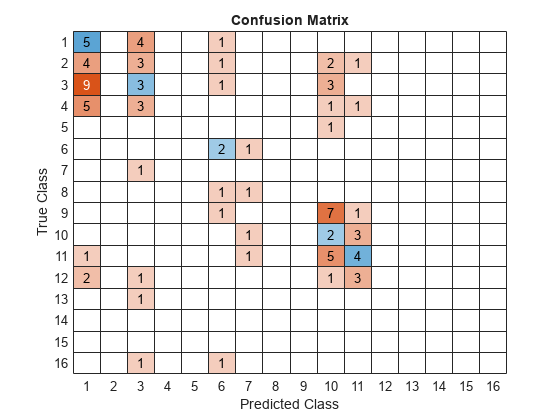
Conclusion and Further Exploration
This example describes the application of a neural network to the beam selection task for a 5G NR system. You can design and train a neural network that outputs a set of good beam pairs. Beam sweeping overhead can be reduced by an exhaustive search only on those selected beam pairs.
The example allows you to specify the scatterers in a MIMO channel. To see the impact of the channel on the beam selection, experiment with different scenarios. The example also provides presaved datasets that can be used to experiment with different network structures and training hyperparameters.
From simulation results, for the prerecorded MIMO scattering channel for 16 beam pairs, the proposed algorithm can achieve a top-K accuracy of 90% when . This indicates with the neural network it is sufficient to perform an exhaustive search over only half of all the beam pairs, reducing the beam sweeping overhead by 50%. Experiment with varying other system parameters to see the efficacy of the network by regenerating data, then retraining and retesting the network.
References
3GPP TR 38.802, "Study on New Radio access technology physical layer aspects." 3rd Generation Partnership Project; Technical Specification Group Radio Access Network.
Klautau, A., González-Prelcic, N., and Heath, R. W., "LIDAR data for deep learning-based mmWave beam-selection," IEEE Wireless Communications Letters, vol. 8, no. 3, pp. 909–912, Jun. 2019.
Heng, Y., and Andrews, J. G., "Machine Learning-Assisted Beam Alignment for mmWave Systems," 2019 IEEE Global Communications Conference (GLOBECOM), 2019, pp. 1-6, doi: 10.1109/GLOBECOM38437.2019.9013296.
Klautau, A., Batista, P., González-Prelcic, N., Wang, Y., and Heath, R. W., "5G MIMO Data for Machine Learning: Application to Beam-Selection Using Deep Learning," 2018 Information Theory and Applications Workshop (ITA), 2018, pp. 1-9, doi: 10.1109/ITA.2018.8503086.
Matteo, Z., <https://github.com/ITU-AI-ML-in-5G-Challenge/PS-012-ML5G-PHY-Beam-Selection_BEAMSOUP> (This is the team achieving the highest test score in the ITU Artificial Intelligence/Machine Learning in 5G Challenge in 2020).
Sim, M. S., Lim, Y., Park, S. H., Dai, L., and Chae, C., "Deep Learning-Based mmWave Beam Selection for 5G NR/6G With Sub-6 GHz Channel Information: Algorithms and Prototype Validation," IEEE Access, vol. 8, pp. 51634-51646, 2020.
Local Function
function prm = validateParams(prm)
% Validate user specified parameters and return updated parameters
%
% Only cross-dependent checks are made for parameter consistency.

    if strcmpi(prm.FreqRange,'FR1')
        if prm.CenterFreq > 7.125e9 || prm.CenterFreq < 410e6
            error(['Specified center frequency is outside the FR1 ', ...
                   'frequency range (410 MHz - 7.125 GHz).']);
        end
        if strcmpi(prm.SSBlockPattern,'Case D') ||  ...
           strcmpi(prm.SSBlockPattern,'Case E')
            error(['Invalid SSBlockPattern for selected FR1 frequency ' ...
                'range. SSBlockPattern must be one of ''Case A'' or ' ...
                '''Case B'' or ''Case C'' for FR1.']);
        end
        if ~((length(prm.SSBTransmitted)==4) || ...
             (length(prm.SSBTransmitted)==8))
            error(['SSBTransmitted must be a vector of length 4 or 8', ...
                   'for FR1 frequency range.']);
        end
        if (prm.CenterFreq <= 3e9) && (length(prm.SSBTransmitted)~=4)
            error(['SSBTransmitted must be a vector of length 4 for ' ...
                   'center frequency less than or equal to 3GHz.']);
        end
        if (prm.CenterFreq > 3e9) && (length(prm.SSBTransmitted)~=8)
            error(['SSBTransmitted must be a vector of length 8 for ', ...
                   'center frequency greater than 3GHz and less than ', ...
                   'or equal to 7.125GHz.']);
        end
    else % 'FR2'
        if prm.CenterFreq > 52.6e9 || prm.CenterFreq < 24.25e9
            error(['Specified center frequency is outside the FR2 ', ...
                   'frequency range (24.25 GHz - 52.6 GHz).']);
        end
        if ~(strcmpi(prm.SSBlockPattern,'Case D') || ...
                strcmpi(prm.SSBlockPattern,'Case E'))
            error(['Invalid SSBlockPattern for selected FR2 frequency ' ...
                'range. SSBlockPattern must be either ''Case D'' or ' ...
                '''Case E'' for FR2.']);
        end
        if length(prm.SSBTransmitted)~=64
            error(['SSBTransmitted must be a vector of length 64 for ', ...
                   'FR2 frequency range.']);
        end
    end

    % Number of beams at transmit/receive ends
    prm.numBeams = sum(prm.SSBTransmitted);

    prm.NumTx = prod(prm.TxArraySize);
    prm.NumRx = prod(prm.RxArraySize);
    if prm.NumTx==1 || prm.NumRx==1
        error(['Number of transmit or receive antenna elements must be', ...
               ' greater than 1.']);
    end
    prm.IsTxURA = (prm.TxArraySize(1)>1) && (prm.TxArraySize(2)>1);
    prm.IsRxURA = (prm.RxArraySize(1)>1) && (prm.RxArraySize(2)>1);

    if ~( strcmpi(prm.RSRPMode,'SSSonly') || ...
          strcmpi(prm.RSRPMode,'SSSwDMRS') )
        error(['Invalid RSRP measuring mode. Specify either ', ...
               '''SSSonly'' or ''SSSwDMRS'' as the mode.']);
    end

    % Select SCS based on SSBlockPattern
    switch lower(prm.SSBlockPattern)
        case 'case a'
            scs = 15;
            cbw = 10;
            scsCommon = 15;
        case {'case b', 'case c'}
            scs = 30;
            cbw = 25;
            scsCommon = 30;
        case 'case d'
            scs = 120;
            cbw = 100;
            scsCommon = 120;
        case 'case e'
            scs = 240;
            cbw = 200;
            scsCommon = 120;
    end
    prm.SCS = scs;
    prm.ChannelBandwidth = cbw;
    prm.SubcarrierSpacingCommon = scsCommon;
end
See Also
Functions
Objects
phased.ULA(Phased Array System Toolbox) |phased.URA(Phased Array System Toolbox) |phased.IsotropicAntennaElement(Phased Array System Toolbox) |dlnetwork
Related Topics
- Deep Learning in MATLAB
- NR SSB Beam Sweeping (5G Toolbox)
