Main Content

fdesign.arbmag

Arbitrary response magnitude filter specification object

Syntax

D= fdesign.arbmag
D= fdesign.arbmag(SPEC)
D = fdesign.arbmag(SPEC,specvalue1,specvalue2,...)
D = fdesign.arbmag(specvalue1,specvalue2,specvalue3)
D = fdesign.arbmag(...,Fs)

Description

D= fdesign.arbmag constructs an arbitrary magnitude filter specification object D.

D= fdesign.arbmag(SPEC) initializes the Specification property to SPEC. The input argument SPEC must be one of the entries shown in the following table. Specification entries are not case sensitive.

Note

Specification entries marked with an asterisk require the DSP System Toolbox™ software.

  • 'N,F,A' — Single band design (default)

  • 'F,A,R' — Single band minimum order design *

  • 'N,B,F,A' — Multiband design

  • 'N,B,F,A,C' — Constrained multiband design *

  • 'B,F,A,R' — Multiband minimum order design *

  • 'Nb,Na,F,A' — Single band design *

  • 'Nb,Na,B,F,A' — Multiband design *

The SPEC entries are defined as follows:

  • A — Amplitude vector. Values in A define the filter amplitude at frequency points you specify in f, the frequency vector. If you use A, you must use F as well. Amplitude values must be real. For complex values designs, use fdesign.arbmagnphase.

  • B — Number of bands in the multiband filter

  • C — Constrained band flag. This enables you to constrain the passband ripple in your multiband design. You cannot constrain the passband ripple in all bands simultaneously.

  • F — Frequency vector. Frequency values in specified in F indicate locations where you provide specific filter response amplitudes. When you provide F, you must also provide A.

  • N — Filter order for FIR filters and the numerator and denominator orders for IIR filters.

  • Nb — Numerator order for IIR filters

  • Na — Denominator order for IIR filter designs

  • R — Ripple

By default, this method assumes that all frequency specifications are supplied in normalized frequency.

Specifying Frequency and Amplitude Vectors

F and A are the input arguments you use to define the filter response desired. Each frequency value you specify in F must have a corresponding response value in A. The following table shows how F and A are related.

Define the frequency vector F as [0 0.25 0.3 0.4 0.5 0.6 0.7 0.75 1.0]

Define the response vector A as [1 1 0 0 0 0 0 1 1]

These specifications connect F and A as shown here:

F (Normalized Frequency)

A (Response Desired at F)

0

1

0.25

1

0.3

0

0.4

0

0.5

0

0.6

0

0.7

0

0.75

1

1.0

1

Different specifications can have different design methods available. Use designmethods to get a list of design methods available for a given specification and filter specification object.

Use designopts to get a list of design options available for a filter specification object and a given design method. Enter help(D,METHOD) to get detailed help on the available design options for a given design method.

D = fdesign.arbmag(SPEC,specvalue1,specvalue2,...) initializes the specifications with specvalue1, specvalue2. Use get(D,'Description') for descriptions of the various specifications specvalue1, specvalue2, ... specvalueN.

D = fdesign.arbmag(specvalue1,specvalue2,specvalue3) uses the default specification 'N,F,A', setting the filter order, filter frequency vector, and the amplitude vector to the values specvalue1, specvalue2, and specvalue3.

D = fdesign.arbmag(...,Fs) specifies the sampling frequency in Hz. All other frequency specifications are also assumed to be in Hz when you specify Fs.

Examples

collapse all

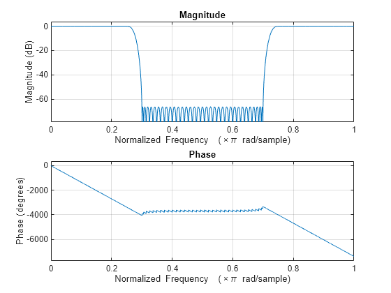
Use fdesign.arbmag to design a three-band filter.

  • Define the frequency vector F = [0 0.25 0.3 0.4 0.5 0.6 0.7 0.75 1.0].

  • Define the response vector A = [1 1 0 0 0 0 0 1 1].

A response with two passbands, one roughly between 0 and 0.25 and the second between 0.75 and 1 results from the mapping between F and A.

N = 150;
B = 3;
F = [0 .25 .3 .4 .5 .6 .7 .75 1];
A = [1 1 0 0 0 0 0 1 1];
A1 = A(1:2);
A2 = A(3:7);
A3 = A(8:end);
F1 = F(1:2);
F2 = F(3:7);
F3 = F(8:end);
d = fdesign.arbmag('N,B,F,A',N,B,F1,A1,F2,A2,F3,A3);
Hd = design(d);
freqz(Hd)

Figure contains 2 axes objects. Axes object 1 with title Phase, xlabel Normalized Frequency (\times\pi rad/sample), ylabel Phase (degrees) contains an object of type line. Axes object 2 with title Magnitude, xlabel Normalized Frequency (\times\pi rad/sample), ylabel Magnitude (dB) contains an object of type line.

Use fdesign.arbmag to design a single band equiripple filter.

Specify 100 frequency points.

n = 120;
f = linspace(0,1,100);

as = ones(1,100)-f*0.2;
absorb = [ones(1,30),1-0.6*bohmanwin(10)',ones(1,5), ...
    1-0.5*bohmanwin(8)',ones(1,47)];
a = as.*absorb;

d = fdesign.arbmag('N,F,A',n,f,a);
hd1 = design(d,'equiripple');

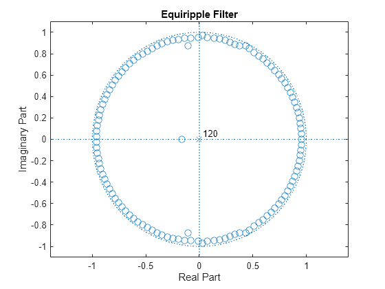
Design a minimum-phase equiripple filter.

hd2 = design(d,'equiripple','MinPhase',true);

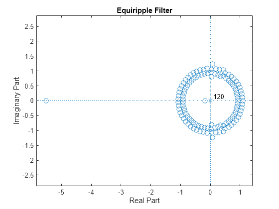
Visualize the poles and zeros of the two filters.

zplane(hd1)
title('Equiripple Filter')

Figure contains an axes object. The axes object with title Equiripple Filter, xlabel Real Part, ylabel Imaginary Part contains 4 objects of type line, text. One or more of the lines displays its values using only markers

zplane(hd2)
title('Equiripple Filter')

Figure contains an axes object. The axes object with title Equiripple Filter, xlabel Real Part, ylabel Imaginary Part contains 4 objects of type line, text. One or more of the lines displays its values using only markers

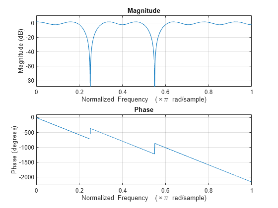
Use fdesign.arbmag to design a multiband minimum order filter.

Place the notches at 0.25π and 0.55π rad/sample.

d = fdesign.arbmag('B,F,A,R');
d.NBands = 5;
d.B1Frequencies = [0 0.2];
d.B1Amplitudes = [1 1];
d.B1Ripple = 0.25;
d.B2Frequencies = 0.25;
d.B2Amplitudes = 0;
d.B3Frequencies = [0.3 0.5];
d.B3Amplitudes = [1 1];
d.B3Ripple = 0.25;
d.B4Frequencies = 0.55;
d.B4Amplitudes = 0;
d.B5Frequencies = [0.6 1];
d.B5Amplitudes = [1 1];
d.B5Ripple = 0.25;
Hd = design(d,'equiripple');

Visualize the frequency response of the resulting filter.

freqz(Hd)

Figure contains 2 axes objects. Axes object 1 with title Phase, xlabel Normalized Frequency (\times\pi rad/sample), ylabel Phase (degrees) contains an object of type line. Axes object 2 with title Magnitude, xlabel Normalized Frequency (\times\pi rad/sample), ylabel Magnitude (dB) contains an object of type line.

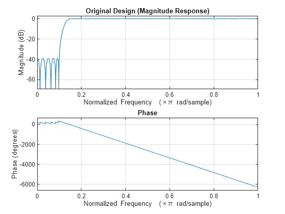
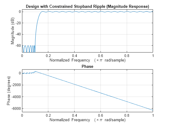
Use fdesign.arbmag to design a multiband constrained FIR filter.

Force the frequency response at 0.15π rad/sample to 0 dB.

d = fdesign.arbmag('N,B,F,A,C',82,2);
d.B1Frequencies = [0 0.06 0.1];
d.B1Amplitudes = [0 0 0];
d.B2Frequencies = [0.15 1];
d.B2Amplitudes = [1 1];

Design a filter with no constraints.

Hd1 = design(d,'equiripple','B2ForcedFrequencyPoints',0.15);

Add a constraint to the first band to increase attenuation.

d.B1Constrained = true;
d.B1Ripple = 0.001;
Hd2 = design(d,'equiripple','B2ForcedFrequencyPoints',0.15);

Visualize the frequency response.

freqz(Hd1);
title('Original Design (Magnitude Response)')

Figure contains 2 axes objects. Axes object 1 with title Phase, xlabel Normalized Frequency (\times\pi rad/sample), ylabel Phase (degrees) contains an object of type line. Axes object 2 with title Original Design (Magnitude Response), xlabel Normalized Frequency (\times\pi rad/sample), ylabel Magnitude (dB) contains an object of type line.

freqz(Hd2);
title('Design with Constrained Stopband Ripple (Magnitude Response)')

Figure contains 2 axes objects. Axes object 1 with title Phase, xlabel Normalized Frequency (\times\pi rad/sample), ylabel Phase (degrees) contains an object of type line. Axes object 2 with title Design with Constrained Stopband Ripple (Magnitude Response), xlabel Normalized Frequency (\times\pi rad/sample), ylabel Magnitude (dB) contains an object of type line.

Version History

Introduced in R2009a