Efficient Narrow Transition-Band FIR Filter Design

Design of a Lowpass Filter with Narrow Transition Bandwidth

One of the drawbacks of using FIR filters is that the filter order tends to grow inversely proportional to the transition bandwidth of the filter. Consider the following design specifications (where the ripples are given in linear units):

Fpass = 2866.5;  % Passband edge
Fstop = 3087;    % Stopband edge
Apass = 0.0174;  % Passband ripple, 0.0174 dB peak to peak
Astop = 66.0206; % Stopband ripple, 66.0206 dB of minimum attenuation
Fs    = 44.1e3;

lowpassSpec = fdesign.lowpass(Fpass,Fstop,Apass,Astop,Fs);

A regular linear-phase equiripple design that meets the specs can be designed with:

eqripFilter = design(lowpassSpec,"equiripple",SystemObject=true);
cost(eqripFilter)

ans = struct with fields:
                  NumCoefficients: 695
                        NumStates: 694
    MultiplicationsPerInputSample: 695
          AdditionsPerInputSample: 694

The filter length required turns out to be 694 taps.

Interpolated FIR (IFIR) Design

The IFIR design algorithm achieves an efficient design for the above specifications in the sense that it reduces the total number of multipliers required. To do this, the design problem is broken into two stages, a filter which is upsampled to achieve the stringent specifications without using many multipliers, and a filter which removes the images created when upsampling the previous filter.

interpFilter = design(lowpassSpec,"ifir",SystemObject=true);

Apparently we have made things worse. Instead of a single filter with 694 multipliers, we now have two filters with a total of 804 multipliers. However, close examination of the second stage shows that only about one multiplier in 5 is non-zero. The actual total number of multipliers has been reduced from 694 to 208.

cost(interpFilter)

ans = struct with fields:
                  NumCoefficients: 208
                        NumStates: 802
    MultiplicationsPerInputSample: 208
          AdditionsPerInputSample: 206

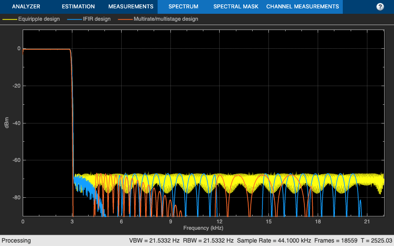
Let's compare the responses of the two designs:

hFiltAnalyzer = filterAnalyzer(eqripFilter,interpFilter);
setLegendStrings(hFiltAnalyzer,["Equiripple design" "IFIR design"])

Manually Controlling the Upsampling Factor

In the previous example, we automatically determined the upsampling factor used such that the total number of multipliers was minimized. It turned out that for the given specifications, the optimal upsampling factor was 5. However, if we examine the design options:

opts = designopts(lowpassSpec,"ifir")

opts = struct with fields:
      FilterStructure: 'dffir'
     UpsamplingFactor: 'auto'
    JointOptimization: 0
         SystemObject: 0

we can see that we can control the upsampling factor. For example, if we wanted to upsample by 4 rather than 5:

opts.UpsamplingFactor = 4;
opts.SystemObject = true; 
upfilter = design(lowpassSpec,"ifir",opts);
cost(upfilter)

ans = struct with fields:
                  NumCoefficients: 217
                        NumStates: 767
    MultiplicationsPerInputSample: 217
          AdditionsPerInputSample: 215

We would obtain a design that has a total of 217 non-zero multipliers.

Using Joint Optimization

It is possible to design the two filters used in IFIR conjunctly. By doing so, we can save a significant number of multipliers at the expense of a longer design time (due to the nature of the algorithm, the design may also not converge altogether in some cases):

opts.UpsamplingFactor = "auto"; % Automatically determine the best factor
opts.JointOptimization = true;
ifirFilter = design(lowpassSpec,"ifir",opts);
cost(ifirFilter)

ans = struct with fields:
                  NumCoefficients: 172
                        NumStates: 726
    MultiplicationsPerInputSample: 172
          AdditionsPerInputSample: 170

For this design, the best upsampling factor found was 6. The number of non-zero multipliers is now only 152

Using Multirate/Multistage Techniques to Achieve Efficient Designs

For the designs discussed so far, single-rate techniques have been used. This means that the number of multiplications required per input sample (MPIS) is equal to the number of non-zero multipliers. For instance, the last design we showed requires 152 MPIS. The single-stage equiripple design we started with required 694 MPIS.

By using multirate/multistage techniques which combine decimation and interpolation we can also obtain efficient designs with a low number of MPIS. For decimators, the number of multiplications required per input sample (on average) is given by the number of multipliers divided by the decimation factor.

multistageFilter = design(lowpassSpec,"multistage",SystemObject=true)

multistageFilter = 
  dsp.FilterCascade with properties:

         Stage1: [1×1 dsp.FIRDecimator]
         Stage2: [1×1 dsp.FIRDecimator]
         Stage3: [1×1 dsp.FIRDecimator]
         Stage4: [1×1 dsp.FIRInterpolator]
         Stage5: [1×1 dsp.FIRInterpolator]
         Stage6: [1×1 dsp.FIRInterpolator]
    CloneStages: true

cost(multistageFilter)

ans = struct with fields:
                  NumCoefficients: 396
                        NumStates: 352
    MultiplicationsPerInputSample: 73
          AdditionsPerInputSample: 70.8333

The first stage has 21 multipliers, and a decimation factor of 3. Therefore, the number of MPIS is 7. The second stage has a length of 45 and a cumulative decimation factor of 6 (that is the decimation factor of this stage multiplied by the decimation factor of the first stage; this is because the input samples to this stage are already coming in at a rate 1/3 the rate of the input samples to the first stage). The average number of multiplications per input sample (reference to the input of the overall multirate/multistage filter) is thus 45/6=7.5. Finally, given that the third stage has a decimation factor of 1, the average number of multiplications per input for this stage is 130/6=21.667. The total number of average MPIS for the three decimators is 36.5.

For the interpolators, it turns out that the filters are identical to the decimators. Moreover, their computational cost is the same. Therefore the total number of MPIS for the entire multirate/multistage design is 73.

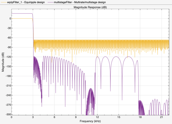
Now we compare the responses of the equiripple design and this one:

hFiltAnalyzer = filterAnalyzer(eqripFilter,multistageFilter)

hFiltAnalyzer = 
  filterAnalyzer with no properties.

setLegendStrings(hFiltAnalyzer,["Equiripple design", "Multirate/multistage design"]);

Notice that the stopband attenuation for the multistage design is about double that of the other designs. This is because it is necessary for the decimators to attenuate out of band components by the required 66 dB in order to avoid aliasing that would violate the required specifications. Similarly, the interpolators need to attenuate images by 66 dB in order to meet the specifications of this problem.

Manually Controlling the Number of Stages

The multirate/multistage design that was obtained consisted of 6 stages. The number of stages is determined automatically by default. However, it is also possible to manually control the number of stages that result. For example:

lp4stage=design(lowpassSpec,"multistage",NStages=4,SystemObject=true);
cost(lp4stage)

ans = struct with fields:
                  NumCoefficients: 516
                        NumStates: 402
    MultiplicationsPerInputSample: 86
          AdditionsPerInputSample: 84.5000

The average number of MPIS for this case is 86

Group Delay

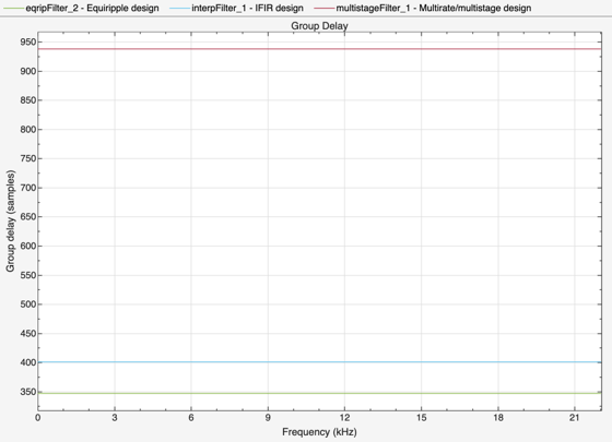
We can compute the group delay for each design. Notice that the multirate/multistage design introduces the most delay (this is the price to pay for a less computationally expensive design). The IFIR design introduces more delay than the single-stage equiripple design, but less so than the multirate/multistage design.

hFiltAnalyzer = filterAnalyzer(eqripFilter,interpFilter,multistageFilter,...
    Analysis="groupdelay");
setLegendStrings(hFiltAnalyzer,["Equiripple design" "IFIR design",...
    "Multirate/multistage design"]);

Filtering a Signal

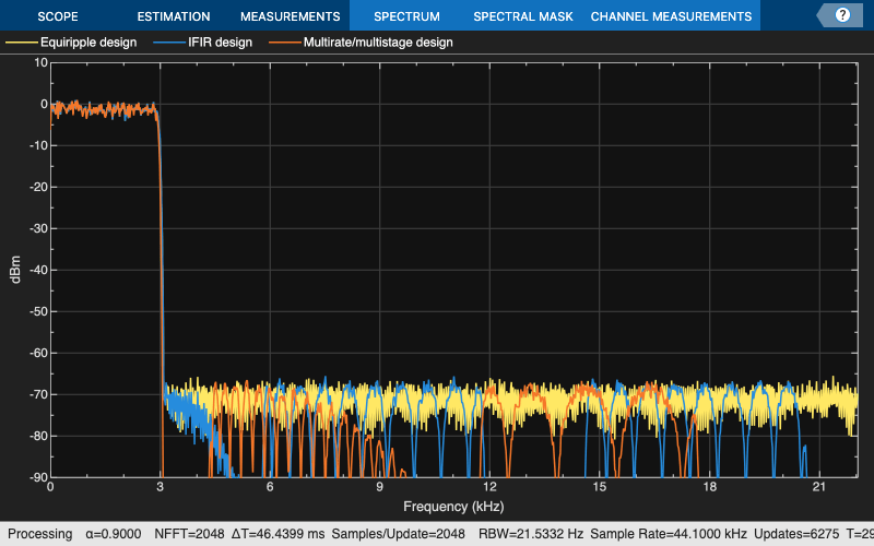
We now show by example that the IFIR and multistage/multirate design perform comparably to the single-stage equiripple design while requiring much less computation. In order to perform filtering for cascades, it is necessary to call generateFilteringCode(ifirFilter) and generateFilteringCode(multistageFilter). This has been done here already in order to create HelperIFIRFilter and HelperMultiFIRFilter.

scope = spectrumAnalyzer(SampleRate=Fs,...
    PlotAsTwoSidedSpectrum=false,YLimits=[-90 10],...
    ShowLegend=true,ChannelNames=["Equiripple design",...
    "IFIR design","Multirate/multistage design"]);
tic,
while toc < 20
    % Run for 20 seconds
    x = randn(6000,1);
    
    % Filter using single stage FIR filter
    y1 = eqripFilter(x);
    
    % Filter using IFIR filter
    y2 = HelperIFIRFilter(x);
    
    % Filter multi-stage/multi-rate FIR filters
    y3 = HelperMultiFIRFilter(x);
    
    % Compare the output from both approaches
    scope([y1,y2,y3])
end