FIR Nyquist (L-th band) Filter Design

Magnitude Response Comparison

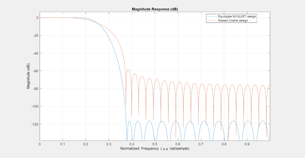
The plot shows the magnitude response of an equiripple Nyquist filter and a raised cosine filter. Both filters have an order of 60 and a rolloff-factor of 0.5. Because the equiripple filter has an optimal equiripple stopband, it has a larger stopband attenuation for the same filter order and transition width. The raised-cosine filter is obtained by truncating the analytical impulse response and it is not optimal in any sense.

NBand = 4;
N = 60;           % Filter order
R = 0.5;          % Rolloff factor
TW = R/(NBand/2); % Transition Bandwidth 
f1 = fdesign.nyquist(NBand,'N,TW',N,TW);
hEq = design(f1,'equiripple',Zerophase=true,SystemObject=true);
coeffs = rcosdesign(R,N/NBand,NBand,'normal');
coeffs = coeffs/max(abs(coeffs))/NBand;
hRC     = dsp.FIRFilter(Numerator=coeffs);
FA = filterAnalyzer(hEq,hRC);
setLegendStrings(FA, ["Equiripple NYQUIST design", "Raised Cosine design"]);

In fact, in this example it is necessary to increase the order of the raised-cosine design to about 1400 in order to attain similar attenuation.

Impulse Response Comparison

Here we compare the impulse responses. Notice that the impulse response in both cases is zero every 4th sample (except for the middle sample). Nyquist filters are also known as L-th band filters, because the cutoff frequency is $\frac{\pi }{\mathit{L}}$ and the impulse response is zero every L-th sample. In this case, we have 4th band filters.

f1.FilterOrder = 38;
hEq1 = design(f1,'equiripple',Zerophase=true,SystemObject=true);
coeffs = rcosdesign(R,f1.FilterOrder/NBand,NBand,'normal');
coeffs = coeffs/max(abs(coeffs))/NBand;
hRC1 = dsp.FIRFilter(Numerator=coeffs);
FA = filterAnalyzer(hEq1,hRC1,Analysis='impulse');

setLegendStrings(FA,["Equiripple NYQUIST","Raised Cosine"]);

Nyquist Filters with a Sloped Stopband

Equiripple designs allow for control of the slope of the stopband of the filter. For example, the following designs have slopes of 0, 20, and 40 dB/(rad/sample)of attenuation:

f1.FilterOrder = 52;
f1.Band = 8;
f1.TransitionWidth = .05;
hEq1 = design(f1,'equiripple', SystemObject=true);
eq2 = design(f1,'equiripple', StopbandShape='linear', StopbandDecay=20,SystemObject=true);
eq3 = design(f1,'equiripple', StopbandShape='linear', StopbandDecay=40,SystemObject=true);
FA = filterAnalyzer(hEq1,eq2,eq3);
setLegendStrings(FA,["Slope=0","Slope=20","Slope=40"]);

Minimum-Phase Design

We can design a minimum-phase spectral factor of the overall Nyquist filter (a square-root in the frequency domain). This spectral factor can be used in a similar manner to the square-root raised-cosine filter in matched filtering applications. A square-root of the filter is placed on the transmitter's end and the other square root is placed at the receiver's end.

f1.FilterOrder = 30;
f1.Band = NBand;
f1.TransitionWidth = TW;
hEq1 = design(f1,'equiripple', Minphase=true, SystemObject=true);
coeffs = rcosdesign(R,N/NBand,NBand);
coeffs = coeffs / max(coeffs) * (-1/(pi*NBand) * (pi*(R-1) - 4*R));
srrc   = dsp.FIRFilter(Numerator=coeffs);
FA = filterAnalyzer(hEq1,srrc);
setLegendStrings(FA,["Minimum-phase equiripple design","Square-root raised-cosine design"]);

Decreasing the Rolloff Factor

The response of the raised-cosine filter improves as the rolloff factor decreases (shown here for rolloff = 0.2). This is because of the narrow main lobe of the frequency response of a rectangular window that is used in the truncation of the impulse response.

f1.FilterOrder = N;
f1.TransitionWidth = .1;
hEq1 = design(f1,'equiripple', Zerophase=true, SystemObject=true);
R = 0.2;
coeffs = rcosdesign(R,N/NBand,NBand,'normal');
coeffs = coeffs/max(abs(coeffs))/NBand;
hRC1   = dsp.FIRFilter(Numerator=coeffs);
FA = filterAnalyzer(hEq1,hRC1);
setLegendStrings(FA,["NYQUIST equiripple design","Raised Cosine design"]);

Windowed-Impulse-Response Nyquist Design

Nyquist filters can also be designed using the truncated-and-windowed impulse response method. This can be another alternative to the raised-cosine design. For example we can use the Kaiser window method to design a filter that meets the initial specs:

f1.TransitionWidth = TW;
kaiserFilt = design(f1, 'kaiserwin', SystemObject=true);

The Kaiser window design requires the same order (60) as the equiripple design to meet the specs. In contrast, we required an extraordinary 1400th-order raised-cosine filter to meet the stopband spec.

FA = filterAnalyzer(hEq,hRC,kaiserFilt);

setLegendStrings(FA,["Equiripple design", "Raised Cosine design", "Kaiser window design"]);

Nyquist Filters for Interpolation

Besides digital data transmission, Nyquist filters are attractive for interpolation purposes. The reason is that every L samples you have a zero sample (except for the middle sample) as mentioned before. There are two advantages to this, both are obvious by looking at the polyphase representation.

fm = fdesign.interpolator(4,'nyquist');
kaiserFilt = design(fm,'kaiserwin',SystemObject=true);
FA = filterAnalyzer(kaiserFilt,PolyphaseDecomposition=true);

The polyphase subfilter #4 is an allpass filter, and in fact, it is a pure delay. To verify that, select impulse response or view the filter coefficients in filterAnalyzer. That pure delay branch of the polyphase filter has the following characteristics: