Fractional Delay Filters Using Farrow Structures

Ideal Fractional Delay Filter

The ideal fractional delay filter is a linear phase allpass filter. Its impulse response is a time-shifted discrete sinc function that corresponds to a noncausal filter. Since the impulse response is infinite, you cannot make it causal by a finite shift in time. The filter therefore cannot be realized and must be approximated.

The Farrow Structure

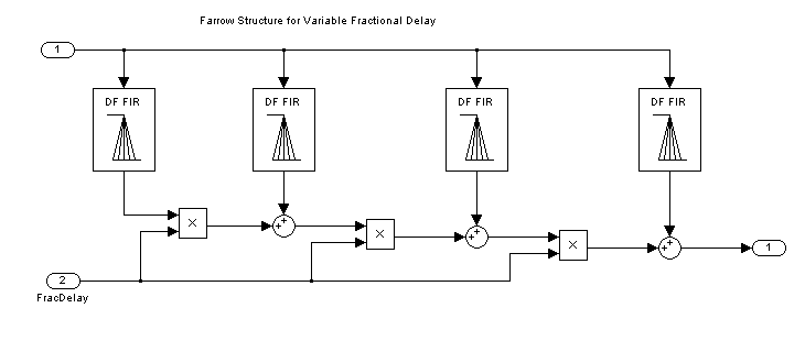
To compute the output of a fractional delay filter, you need to estimate the values of the input signal between the existing discrete-time samples. You can use special interpolation filters to compute new sample values at arbitrary points. Among interpolation filters, polynomial-based filters are of particular interest because a special structure—the Farrow structure—permits a simpler handling of coefficients. In particular, the tunability of the Farrow structure makes it well suited for practical hardware implementations.

Maximally Flat FIR Approximation (Lagrange Interpolation)

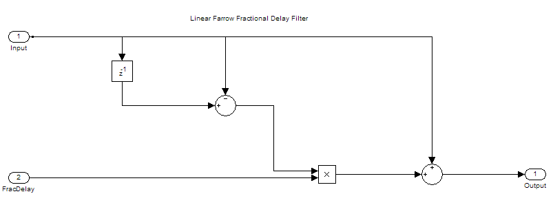
Lagrange interpolation is a time-domain approach that leads to a special case of polynomial-based filters, where you approximare the output signal with a polynomial of degree M. The simplest case (M = 1) corresponds to linear interpolation. Design and analyze a linear fractional delay filter that splits the unit delay by various fractions.

Nx = 1024;
Nf = 5;
yw = zeros(Nx,Nf);
transferFuncEstimator = dsp.TransferFunctionEstimator( ...
    SpectralAverages=25,FrequencyRange="onesided");
arrPlotPhaseDelay = dsp.ArrayPlot(PlotType="Line",YLimits=[0 1.5], ...
    YLabel="Phase delay",SampleIncrement=1/512);
arrPlotMag = dsp.ArrayPlot(PlotType="Line",YLimits=[-10 1], ...
    YLabel="Magnitude (dB)",SampleIncrement=1/512);

fracDelay = dsp.VariableFractionalDelay;

xw = randn(Nx,Nf);
transferFuncEstimator(xw,yw);
w = getFrequencyVector(transferFuncEstimator,2*pi);
w = repmat(w,1,Nf);
tic,
while toc < 2 
    yw = fracDelay(xw,[0 0.2 0.4 0.6 0.8]); 
    H = transferFuncEstimator(xw,yw); 
    arrPlotMag(20*log10(abs(H))) 
    arrPlotPhaseDelay(-angle(H)./w) 
end 
release(fracDelay)
release(transferFuncEstimator)
release(arrPlotMag)

release(arrPlotPhaseDelay)

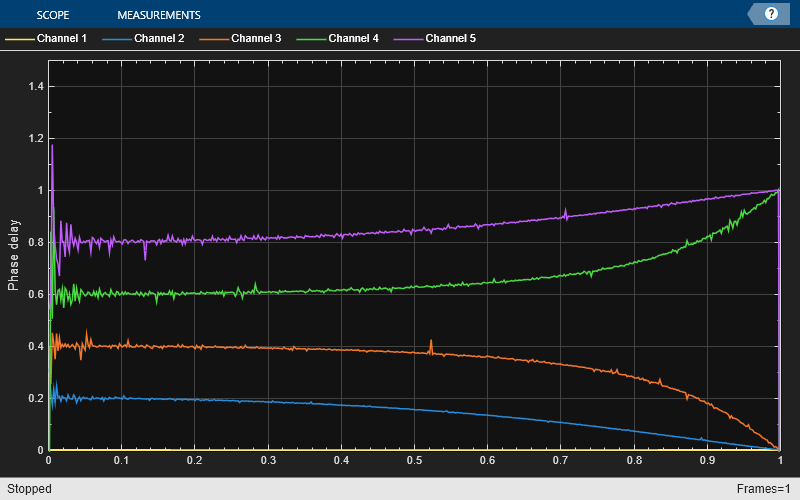
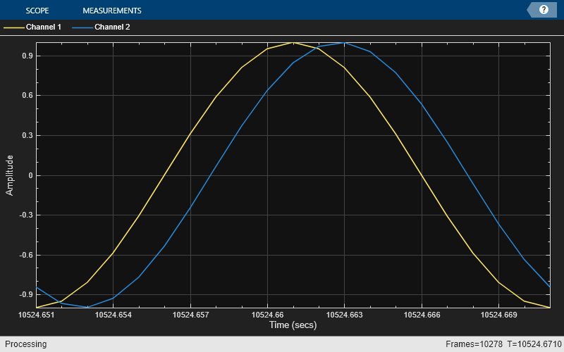
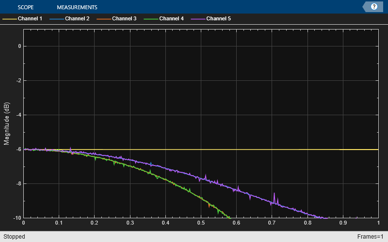
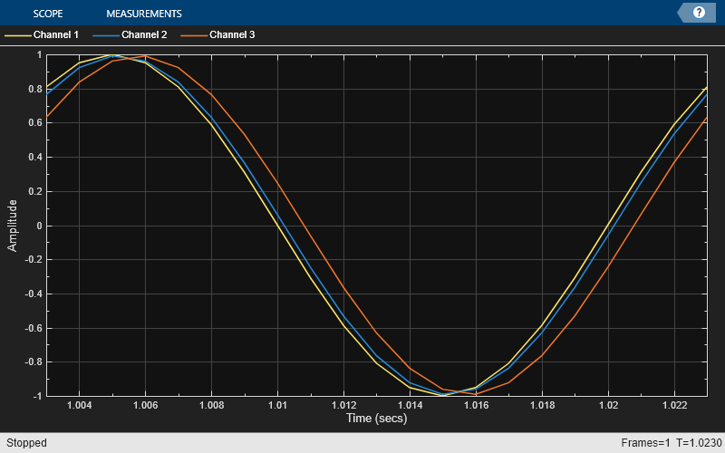
For any delay value, the ideal filter should have both a flat magnitude response and a flat phase delay response. The approximation is correct only for the lowest frequencies. Hence, in practice, you need to oversample the signals for the linear fractional delay to work correctly. In this step, you apply two different fractional delays to a sine wave and use the time scope to overlay the original sine wave and the two delayed versions. A delay of 0.2 samples with a sample rate of 1000 Hz corresponds to a delay of 0.2 ms.

scope = timescope(SampleRate=1000, ...
                  YLimits=[-1 1], ...
                  TimeSpan=.02, ...
                  TimeSpanOverrunAction="scroll");
sine = dsp.SineWave(Frequency=50, SamplesPerFrame=Nx);
tic,
while toc < 2
    x  = sine();
    y = fracDelay(x,[.2 .8]); % Delay by 0.2 and 0.8 samples (i.e. 0.2ms and 0.8ms respectively)
    scope([x,y(:,1),y(:,2)])
end
release(fracDelay)
release(scope);

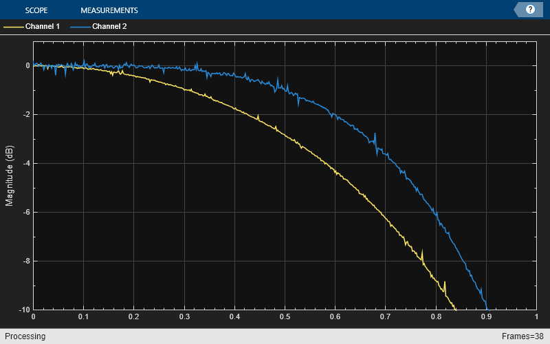
You can design higher order Lagrange interpolators. Compare a cubic Lagrange interpolator with a linear one.

farrowFracDelay = dsp.VariableFractionalDelay( ...
    InterpolationMethod="Farrow",MaximumDelay=1025);
Nf = 2;
yw = zeros(Nx,Nf);
xw = randn(Nx,Nf);
H = transferFuncEstimator(xw,yw);
w = getFrequencyVector(transferFuncEstimator,2*pi);
w = repmat(w,1,Nf);
tic,
while toc < 2
    % Run for 2 seconds
    yw(:,1) = fracDelay(xw(:,1),0.4);  % Delay by 0.4 samples (0.4ms)
    yw(:,2) = farrowFracDelay(xw(:,2),1.4); % Delay by 1.4 samples (1.4ms)  
    H = transferFuncEstimator(xw,yw);    
    arrPlotMag(20*log10(abs(H)))
    arrPlotPhaseDelay(-unwrap(angle(H))./w)
end 
release(fracDelay)
release(transferFuncEstimator)
release(arrPlotMag)

release(arrPlotPhaseDelay)

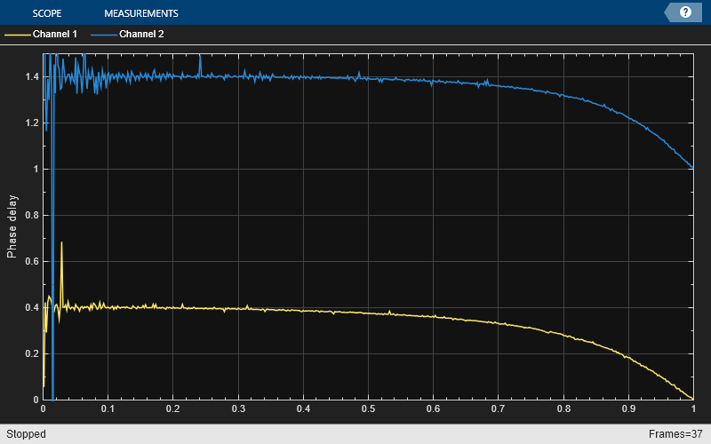
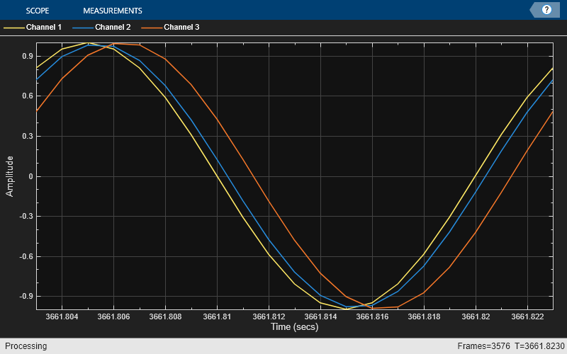
Increasing the order of the polynomials slightly increases the useful bandwidth when you are using Lagrange approximation. The length of the differentiating filters, that is, the number of pieces of the impulse response (number of rows in the 'Coefficients' property) is equal to the length of the polynomials (number of columns in the 'Coefficients' property). You can use other design methods to overcome this limitation. The phase delay of the third-order filter shifts from 0.4 to 1.4 samples at DC. Since the cubic Lagrange interpolator is a third-order filter, the minimum delay it can achieve is 1. For this reason, the delay is 1.4 ms instead of 0.4 ms for this case.

sine = dsp.SineWave(Frequency=50,SamplesPerFrame=Nx);
tic,
while toc < 2
       x  = sine();
       y1 = fracDelay(x,0.4);
       y2 = farrowFracDelay(x,1.4);
       scope([x,y1,y2])
end
release(fracDelay)
release(scope);

Time-Varying Fractional Delay

The advantage of the Farrow structure over a direct-form FIR resides in its tunability. In many practical applications, the delay is time varying. For each new delay, you would need a new set of coefficients in the direct-form implementation, but with a Farrow implementation, the polynomial coefficients remain constant.

tic,
while toc < 5
    x  = sine();
    if toc < 1
        delay = 1;
    elseif toc < 2
        delay = 1.2;
    elseif toc < 3
        delay = 1.4;
    elseif toc < 4
        delay = 1.6;
    else
        delay = 1.8;
    end
    y = farrowFracDelay(x,delay); 
    scope([x,y])
end
release(fracDelay)
release(scope);