High Resolution Spectral Analysis in MATLAB

Resolution in Spectral Analysis

Resolution in this context refers to the ability to distinguish between two spectral components that lie in the vicinity of each other. Resolution depends on the length of the time-domain segment used to compute the spectrum. When windowing is used on the time-domain segment as is the case with modified periodograms, the type of window used also affects the resolution.

The classical tradeoff with different windows is one of resolution vs. sidelobe attenuation. Rectangular windows provide the highest resolution but very poor (~14 dB) sidelobe attenuation. Poor sidelobe attenuation can result in spectral components being buried by the windowing operation and thus is undesirable. Hann windows provide good sidelobe attenuation at the expense of lower frequency resolution. Parameterizable windows such as Kaiser allow to control the tradeoff by changing the window parameter.

Instead of using averaged modified periodograms (Welch's method), a higher resolution estimate can be achieved by using a filter bank approach that emulates how analog spectrum analyzers work. The main idea is to divide the signal into different frequency bins using a filter bank and computing the average power of each subband signal.

Filter Bank-Based Spectrum Estimation

For this example, 512 different bandpass filters need to be used to get the same resolution afforded by the rectangular window. In order to implement the 512 bandpass filters efficiently, a polyphase analysis filter bank (a.k.a. channelizer) is used. This works by taking a prototype lowpass filter with a bandwidth of Fs/N where N the desired frequency resolution (512 in this example), and implementing the filter in polyphase form much like an FIR decimator is implemented. Instead of adding the results of all the branches as in the decimator case, each branch is used as an input to an N-point FFT. It can be shown that each output of the FFT corresponds a modulated version of a lowpass filter, thus implementing a bandpass filter. The main drawback of the filter bank approach is increased computation due to the polyphase filter as well as slower adaptation to changing signals due to the states of that filter. More details can be found in the book 'Multirate Signal Processing for Communications Systems' by fredric j. harris. Prentice Hall PTR, 2004.

In this example, 100 averages of the spectrum estimate are used throughout. The sampling frequency is set to 1 MHz. It is assumed that we are working with frames of 64 samples which will need to be buffered in order to perform the spectrum estimation.

NAvg = 100;
Fs = 1e6;
FrameSize = 64;
NumFreqBins = 512;
filterBankRBW = Fs/NumFreqBins;

spectrumAnalyzer implements a filter bank-based spectrum estimator when Method is set accordingly. Internally, it uses dsp.Channelizer which implements the polyphase filtering plus FFT (and can be used for other applications besides spectrum analysis, e.g. multicarrier communications).

filterBankSA = spectrumAnalyzer(...
    'SampleRate',Fs,...
    'RBWSource','property',...
    'RBW',filterBankRBW,...
    'AveragingMethod','exponential', ...
    'ForgettingFactor',0.001, ...
    'PlotAsTwoSidedSpectrum',false,...
    'YLimits',[-150 50],...
    'YLabel','Power',...
    'Title','Filter bank Power Spectrum Estimate',...
    'Position',[50 375 800 450]);

Test Signal

In this example, the test signal is acquired in 64-sample frames. For spectral analysis purposes, the larger the frame, the better the resolution.

The test signal consists of two sine waves plus white Gaussian noise. Changing the number of frequency bins, amplitude, frequency, and noise power values is instructive and encouraged.

sinegen = dsp.SineWave('SampleRate',Fs,...
    'SamplesPerFrame',FrameSize);

Initial Test Case

To start, compute the filter bank spectral estimate for sine waves of amplitude 1 and 2 and frequencies of 200 kHz and 250 kHz, respectively. The white Gaussian noise has an average power (variance) of 1e-12. Note that the onesided noise floor of -114 dBm is accurately shown in the spectral estimate.

release(sinegen)
sinegen.Amplitude = [1 2];
sinegen.Frequency = [200000 250000];

noiseVar = 1e-12;
% -114 dBm onesided
noiseFloor = 10*log10((noiseVar/(NumFreqBins/2))/1e-3); 
fprintf('Noise Floor\n');

Noise Floor

fprintf('Filter bank noise floor = %.2f dBm\n\n',noiseFloor);

Filter bank noise floor = -114.08 dBm

timesteps = 10 * ceil(NumFreqBins / FrameSize);
for t = 1:timesteps
    x = sum(sinegen(),2) + sqrt(noiseVar)*randn(FrameSize,1);
    filterBankSA(x);
end

release(filterBankSA)

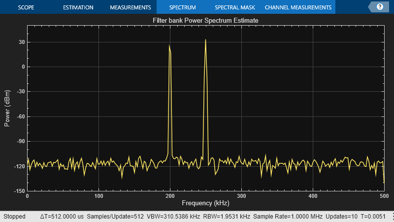
Numerical Computation Using Spectrum Estimator

dsp.SpectrumEstimator can be used to compute the filter bank spectrum estimates.

In order to feed the spectrum estimator a longer frame, a buffer gathers 512 samples before computing the spectral estimate. Although not used in this example, the buffer allows for overlapping which can be used to increase the number of averages obtained from a given set of data.

filterBankEstimator = dsp.SpectrumEstimator(...
    'Method','Filter bank',...
    'AveragingMethod','Exponential', ...
    'ForgettingFactor',0.7, ...
    'SampleRate',Fs,...
    'FrequencyRange','onesided',...
    'PowerUnits','dBm');

buff    = dsp.AsyncBuffer;

release(sinegen)

timesteps = 10 * ceil(NumFreqBins / FrameSize);
for t = 1:timesteps 
    x     = sum(sinegen(),2) + sqrt(noiseVar)*randn(FrameSize,1);
    write(buff,x);      % Buffer data
    if buff.NumUnreadSamples >= NumFreqBins
        xbuff = read(buff,NumFreqBins);
        Pfbse = filterBankEstimator(xbuff);
    end
end

Compare Spectrum Estimates Using Different Methods

Compute the welch and the filter bank spectral estimate for sine waves of amplitude 1 and 2 and frequencies of 200 kHz and 250 kHz, respectively. The white Gaussian noise has an average power (variance) of 1e-12.

release(sinegen)
sinegen.Amplitude = [1 2];
sinegen.Frequency = [200000 250000];

filterBankSA.RBWSource = 'auto';
filterBankSA.ForgettingFactor = 0.7;
filterBankSA.Position = [50 375 400 450];

welchSA = spectrumAnalyzer(...
    'Method','welch',...
    'SampleRate',Fs,...
    'PlotAsTwoSidedSpectrum',false,...
    'YLimits',[-150 50],...
    'YLabel','Power',...
    'Title','Welch Power Spectrum Estimate',...
    'Position',[450 375 400 450]);

noiseVar = 1e-12;

timesteps = 500 * ceil(NumFreqBins / FrameSize);
for t = 1:timesteps
    x = sum(sinegen(),2) + sqrt(noiseVar)*randn(FrameSize,1);
    filterBankSA(x);
    welchSA(x);
end

release(filterBankSA)

RBW = 488.28;
hannNENBW = 1.5;

welchNSamplesPerUpdate = Fs*hannNENBW/RBW;
filterBankNSamplesPerUpdate = Fs/RBW;

fprintf('Samples/Update\n');

Samples/Update

fprintf('Welch Samples/Update = %.3f Samples\n',...
    welchNSamplesPerUpdate);

Welch Samples/Update = 3072.008 Samples

fprintf('Filter bank Samples/Update = %.3f Samples\n\n',...
    filterBankNSamplesPerUpdate);

Filter bank Samples/Update = 2048.005 Samples

welchNoiseFloor = 10*log10((noiseVar/(welchNSamplesPerUpdate/2))/1e-3);
filterBankNoiseFloor = 10*log10((noiseVar/(filterBankNSamplesPerUpdate/2))/1e-3);

fprintf('Noise Floor\n');

Noise Floor

fprintf('Welch noise floor       = %.2f dBm\n',welchNoiseFloor);

Welch noise floor       = -121.86 dBm

fprintf('Filter bank noise floor = %.2f dBm\n\n',filterBankNoiseFloor);

Filter bank noise floor = -120.10 dBm

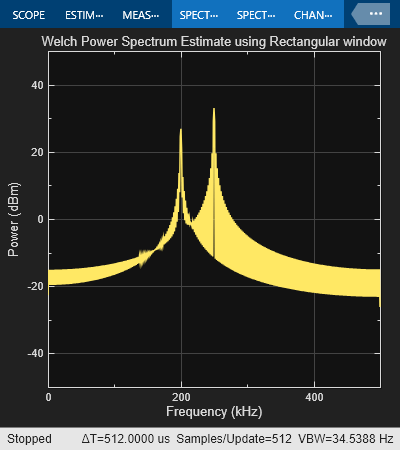
Both Welch and Filter bank-based spectrum estimate detected the two tones at 200 kHz and 250 kHz. Filter bank-based spectrum estimate has better isolation of tones. For the same Resolution Bandwidth (RBW), averaged modified periodogram (Welch's) method requires 3073 samples to compute the spectrum compared to 2048 required by filter bank-based estimate. Note that the onesided noise floor of -120 dBm is accurately shown in the filter bank spectral estimate.

Compare Modified Periodograms Using Different Windows

Consider two spectrum analyzers in which the only difference is the window used: rectangular or Hann.

rectRBW = Fs/NumFreqBins;
hannNENBW = 1.5;
hannRBW = Fs*hannNENBW/NumFreqBins;

rectangularSA = spectrumAnalyzer(...
    'Method','welch', ...
    'SampleRate',Fs,...
    'Window','rectangular',...
    'RBWSource','property',...
    'RBW',rectRBW,...
    'PlotAsTwoSidedSpectrum',false,...
    'YLimits',[-50 50],...
    'YLabel','Power',...
    'Title','Welch Power Spectrum Estimate using Rectangular window',...
    'Position',[50 375 400 450]);

hannSA = spectrumAnalyzer(...
    'Method','welch', ...
    'SampleRate',Fs,...
    'Window','hann',...
    'RBWSource','property',...
    'RBW',hannRBW,...
    'PlotAsTwoSidedSpectrum',false,...
    'YLimits',[-150 50],...
    'YLabel','Power',...
    'Title','Welch Power Spectrum Estimate using Hann window',...
    'Position',[450 375 400 450]);

release(sinegen)
sinegen.Amplitude = [1 2]; % Try [0 2] as well
sinegen.Frequency = [200000 250000];

noiseVar = 1e-12;
timesteps = 10 * ceil(NumFreqBins / FrameSize);
for t = 1:timesteps 
    x = sum(sinegen(),2) + sqrt(noiseVar)*randn(FrameSize,1);
    rectangularSA(x);
    hannSA(x);
end
release(rectangularSA)

release(hannSA)

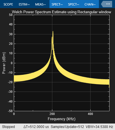
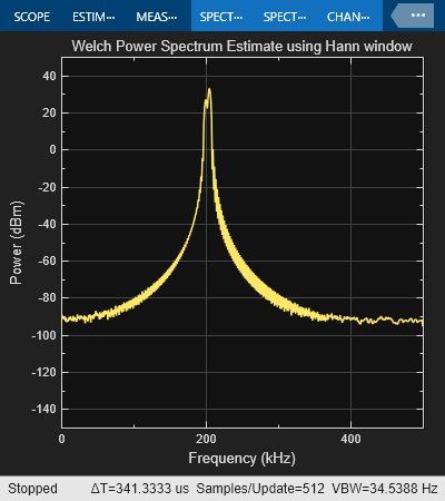
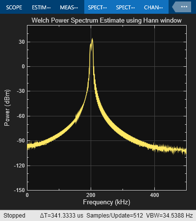
The rectangular window provides a narrow mainlobe at the expense of low sidelobe attenuation. In contrast, the Hann window provides a broader mainlobe in exchange for the much larger sidelobe attenuation. The broader mainlobe is particularly noticeable at 250 kHz. Both windows exhibit large rolloffs around the frequencies at which the sine waves lie. This can mask low power signals of interest above the noise floor. That problem is virtually non-existent in the filter bank case.

Changing the amplitudes to [0 2] rather than [1 2] effectively means there is a single sine wave of 250 kHz along with noise. This case is interesting because the rectangular window behaves particularly well when the 200 kHz sine wave is not interfering. The reason is that 250 kHz is one of the 512 frequencies that divide 1 MHz evenly. In that case, the time domain replicas introduced by the frequency sampling inherent in the FFT make a perfect periodic extension of the time-limited data segment used for the power spectrum computation. In general, for sine waves with arbitrary frequencies, this is not the case. This dependence on the frequency of the sine wave along with the susceptibility to signal interference is another drawback of the modified periodogram approach.

Resolution Bandwidth (RBW)

The resolution bandwidth for each analyzer can be computed once the input length is known. The RBW indicates the bandwidth over which the power component is computed. That is to say, each element of the power spectrum estimate represents the power in Watts, dBW, or dBm across a bandwidth of width RBW centered around the frequency corresponding to the element of the estimate. The power value of each element in the power spectrum estimate is found by integrating the power-density over the frequency band spanned by the RBW value. A lower RBW indicates a higher resolution since the power is computed over a finer grid (a smaller bandwidth). Rectangular windows have the highest resolution of all windows. In the case of the Kaiser window, the RBW depends on the sidelobe attenuation used.

fprintf('RBW\n')

RBW

fprintf('Welch-Rectangular  RBW = %.3f Hz\n',rectRBW);

Welch-Rectangular  RBW = 1953.125 Hz

fprintf('Welch-Hann         RBW = %.3f Hz\n',hannRBW);

Welch-Hann         RBW = 2929.688 Hz

fprintf('Filter bank        RBW = %.3f Hz\n\n',filterBankRBW);

Filter bank        RBW = 1953.125 Hz

In the case of setting the amplitudes to [0 2], i.e. the case in which there is a single sine wave at 250 kHz, it is interesting to understand the relation between the RBW and the noise floor. The expected noise floor is 10*log10((noiseVar/(NumFreqBins/2))/1e-3) or about -114 dBm. The spectral estimate corresponding to the rectangular window has the expected noise floor, but the spectral estimate using the Hann window has a noise floor that is about 2 dBm higher than expected. The reason for this is that the spectral estimate is compute at 512 frequency points but the power spectrum is integrated over the RBW of the particular window. For the rectangular window, the RBW is exactly 1 MHz/512 so that the spectral estimate contains independent estimates of the power for each frequency bin. For the Hann window, the RBW is larger, so that the spectral estimate contains overlapping power from one frequency bin to the next. This overlapping power increases the power value in each bin and elevates the noise floor. The amount can be computed analytically as follows:

hannNoiseFloor = 10*log10((noiseVar/(NumFreqBins/2)*hannRBW/rectRBW)/1e-3);
fprintf('Noise Floor\n');

Noise Floor

fprintf('Hann noise floor = %.2f dBm\n\n',hannNoiseFloor);

Hann noise floor = -112.32 dBm

Sinusoids in Close Proximity to Each Other

To illustrate the resolution issue consider the following case. The sinusoid frequencies are changed to 200 kHz and 205 kHz. The filter bank estimate remains accurate. Focusing on the window-based estimators, because of the broader mainlobe in the Hann window, the two sinusoids are harder to distinguish when compared to the rectangular window estimate. The fact is that neither of the two estimates is particularly accurate. Note that 205 kHz is basically at the limit of what we can distinguish from 200 kHz. For closer frequencies, all three estimators will fail to separate the two spectral components. The only way to separate closer components is to have larger frame sizes and therefore a larger number of NumFrequencyBands in the case of the filter bank estimator.

release(sinegen)
sinegen.Amplitude = [1 2];
sinegen.Frequency = [200000 205000];

filterBankSA.RBWSource = 'property';
filterBankSA.RBW       =  filterBankRBW;
filterBankSA.Position  = [850 375 400 450];

noiseVar = 1e-10;
noiseFloor = 10*log10((noiseVar/(NumFreqBins/2))/1e-3); % -94 dBm onesided
fprintf('Noise Floor\n');

Noise Floor

fprintf('Noise floor = %.2f dBm\n\n',noiseFloor);

Noise floor = -94.08 dBm

timesteps = 500 * ceil(NumFreqBins / FrameSize);
for t = 1:timesteps 
    x  = sum(sinegen(),2) + sqrt(noiseVar)*randn(FrameSize,1);
    filterBankSA(x);
    rectangularSA(x);
    hannSA(x);
end

release(filterBankSA)

release(rectangularSA)

release(hannSA)

Detecting Low Power Sinusoidal Components

Next, re-run the previous scenario but add a third sinusoid at 170 kHz with a very small amplitude. This third sinusoid is missed completely by the rectangular window estimate and the Hann window estimate. The filter bank estimate provides both better resolution and better isolation of tones, so that the three sine waves are clearly visible.

release(sinegen)
sinegen.Amplitude = [1e-5 1 2];
sinegen.Frequency = [170000 200000 205000];

noiseVar = 1e-11;
noiseFloor = 10*log10((noiseVar/(NumFreqBins/2))/1e-3); % -104 dBm onesided
fprintf('Noise Floor\n');

Noise Floor

fprintf('Noise floor = %.2f dBm\n\n',noiseFloor);

Noise floor = -104.08 dBm

timesteps = 500 * ceil(NumFreqBins / FrameSize);
for t = 1:timesteps 
    x  = sum(sinegen(),2) + sqrt(noiseVar)*randn(FrameSize,1);
    filterBankSA(x);
    rectangularSA(x);
    hannSA(x);
end

release(filterBankSA)

release(rectangularSA)

release(hannSA)