Least Pth-Norm Optimal IIR Filter Design

IIRLPNORM Fundamentals

The iirlpnorm algorithm differs from the traditional IIR design algorithms in several aspects:

Lowpass Design

For simple designs such as lowpass and highpass, specify passband and stopband frequencies. The transition band is considered as a don't-care band by the algorithm.

d = fdesign.lowpass('N,Fp,Fst',8,.4,.5) 

d = 
  lowpass with properties:

               Response: 'Lowpass'
          Specification: 'N,Fp,Fst'
            Description: {3x1 cell}
    NormalizedFrequency: 1
            FilterOrder: 8
                  Fpass: 0.4000
                  Fstop: 0.5000

hiirlpnorm = design(d,'iirlpnorm','SystemObject',true);

For comparison purposes, consider this elliptic filter design.

d = fdesign.lowpass('N,Fp,Ap,Ast',8,.4,0.0084,66.25);
hellip = design(d,'ellip','SystemObject',true)

hellip = 
  dsp.SOSFilter with properties:

            Structure: 'Direct form II'
    CoefficientSource: 'Property'
            Numerator: [4x3 double]
          Denominator: [4x3 double]
       HasScaleValues: true
          ScaleValues: [0.7442 0.7330 1.4088 0.0154 1]

  Use get to show all properties

hfvt = fvtool(hiirlpnorm,hellip);
legend(hfvt,'IIRLPNORM design','ELLIP design');

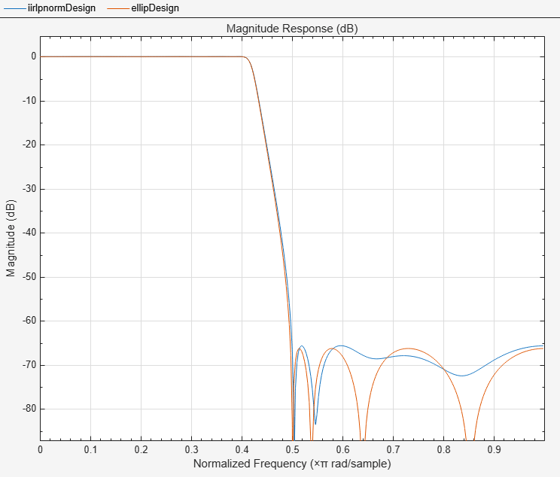
The response of the two filters is very similar. Zooming into the passband accentuates the point. However, the magnitude of the filter designed with iirlpnorm is not constrained to be less than 0 dB.

zoom(hfvt,[0 .44 -.0092 .0052]);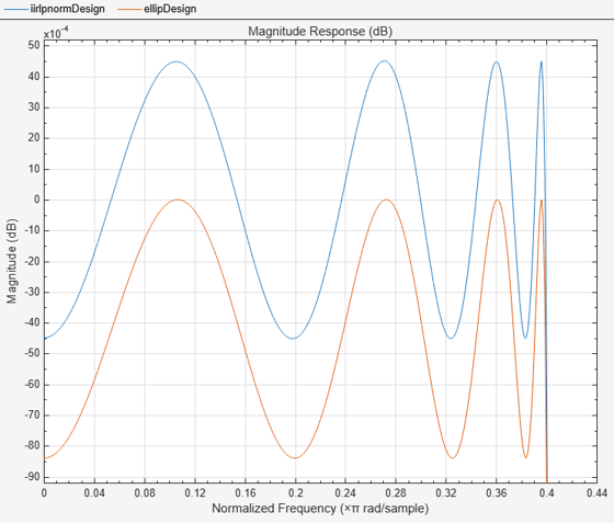

Different Numerator and Denominator Orders

While we can get very similar designs with elliptic filters, iirlpnorm algorithm provides greater flexibility. For instance the denominator can be set different than numerator.

d = fdesign.lowpass('Nb,Na,Fp,Fst',8,6,.4,.5) 

d = 
  lowpass with properties:

               Response: 'Lowpass'
          Specification: 'Nb,Na,Fp,Fst'
            Description: {4x1 cell}
    NormalizedFrequency: 1
               NumOrder: 8
               DenOrder: 6
                  Fpass: 0.4000
                  Fstop: 0.5000

hiirlpnorm = design(d,'iirlpnorm','SystemObject',true);

With elliptic filters (and other classical IIR designs), we must change both the numerator and the denominator order.

d = fdesign.lowpass('N,Fp,Ap,Ast',6,.4,0.0084,58.36);
hellip = design(d,'ellip','SystemObject',true);
hfvt = fvtool(hiirlpnorm,hellip);
legend(hfvt,'IIRLPNORM design','ELLIP design');

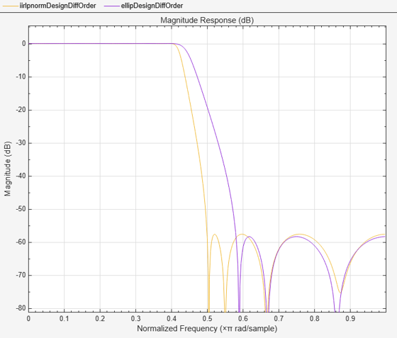
Clearly, the elliptic design (in green) now results in a much wider transition width.

Weighting the Designs

Similar to equiripple or least-square designs, we can weight the optimization criteria to alter the design as we see fit. However, unlike equiripple, we have the extra flexibility of providing different weights for each frequency point instead of for each frequency band.

Consider the following two highpass filters:

d = fdesign.highpass('Nb,Na,Fst,Fp',6,4,.6,.7) 

d = 
  highpass with properties:

          Specification: 'Nb,Na,Fst,Fp'
               Response: 'Highpass'
            Description: {4x1 cell}
    NormalizedFrequency: 1
               NumOrder: 6
               DenOrder: 4
                  Fstop: 0.6000
                  Fpass: 0.7000

h1 = design(d,'iirlpnorm','Wpass',1,'Wstop',10,'SystemObject',true);
h2 = design(d,'iirlpnorm','Wpass',1,'Wstop',[100 10],'SystemObject',true);
hfvt = fvtool(h1,h2);
legend(hfvt,'Same weight for entire band',...
    'Different weights in stopband');

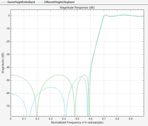
The first design uses the same weight per band (10 in the stopband, 1 in the passband). The second design uses a different weight per frequency point. This provides a simple way of attaining a sloped stopband which may be desirable in some applications. The extra attenuation over portions of the stopband comes at the expense of a larger passband ripple and transition width.

The Pth-Norm

Roughly speaking, the optimal design is achieved by minimizing the error between the actual designed filter and an ideal filter in the Pth-norm sense. Different values of the norm result in different designs. When specifying the P-th norm, we actually specify two values, 'InitNorm' and 'Norm' where 'InitNorm' is the initial value of the norm used by the algorithm and 'Norm' is the final (the actual) value for which the design is optimized. Starting the optimization with a smaller initial value aids in the convergence of the algorithm.

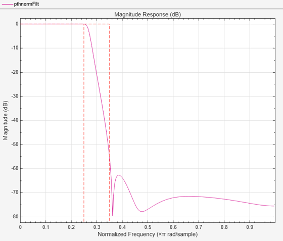
By default, the algorithm starts optimizing in the 2-norm sense but finally optimizes the design in the 128-norm sense. The 128-norm in practice yields a good approximation to the infinity-norm. So that the designs tend to be equiripple. For a least-squares design, we should set the norm to 2. For instance, consider the following lowpass filter

d = fdesign.lowpass('Nb,Na,Fp,Fst',10,7,.25,.35);
design(d,'iirlpnorm','Norm',2,'SystemObject',true);

Arbitrary Shaped Magnitude

Another of the important features of iirlpnorm is its ability to design filters other than the basic lowpass, highpass, bandpass and bandstop filters. See the Arbitrary Magnitude Filter Design example for more information. We now show a few examples: Rayleigh Fading Channel and Optical Absorption of Atomic Rubidium87 Vapor.

Rayleigh Fading Channel

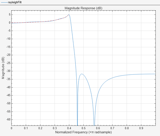
Here's a filter for noise shaping when simulating a Rayleigh fading wireless communications channel

F1 = 0:0.01:0.4;
A1 = 1.0 ./ (1 - (F1./0.42).^2).^0.25;
F2 = [0.45 1];
A2 = [0 0];
d = fdesign.arbmag('Nb,Na,B,F,A',4,6,2,F1,A1,F2,A2);
design(d,'iirlpnorm','SystemObject',true);

fig = gcf;
fig.Color = [1 1 1];

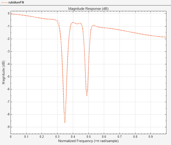
Optical Absorption of Atomic Rubidium87 Vapor

The following design models the absorption of light in a certain gas. The resulting filter turns out to have approximately linear-phase:

Nb = 12;
Na = 10;
F = linspace(0,1,100);
As = ones(1,100)-F*0.2;
Absorb = [ones(1,30),(1-0.6*bohmanwin(10))', ...
    ones(1,5), (1-0.5*bohmanwin(8))',ones(1,47)];
A = As.*Absorb;
d = fdesign.arbmag('Nb,Na,F,A',Nb,Na,F,A);
W = [ones(1,30) ones(1,10)*.2 ones(1,60)];
design(d,'iirlpnorm','Weights',W,'Norm',2,'DensityFactor',30, ...
    'SystemObject',true);