System Identification of FIR Filter Using Normalized LMS Algorithm
To improve the convergence performance of the LMS algorithm, the normalized variant (NLMS) uses an adaptive step size based on the signal power. As the input signal power changes, the algorithm calculates the input power and adjusts the step size to maintain an appropriate value. The step size changes with time, and as a result, the normalized algorithm converges faster with fewer samples in many cases. For input signals that change slowly over time, the normalized LMS algorithm can be a more efficient LMS approach.
For an example using the LMS approach, see System Identification of FIR Filter Using LMS Algorithm.
Unknown System
Create a dsp.FIRFilter object that represents the system to be identified. Use the fircband function to design the filter coefficients. The designed filter is a lowpass filter constrained to 0.2 ripple in the stopband.
filt = dsp.FIRFilter;
filt.Numerator = fircband(12,[0 0.4 0.5 1],[1 1 0 0],[1 0.2],...
{'w' 'c'});
Pass the signal x to the FIR filter. The desired signal d is the sum of the output of the unknown system (FIR filter) and an additive noise signal n.
x = 0.1*randn(1000,1);
n = 0.001*randn(1000,1);
d = filt(x) + n;
Adaptive Filter
To use the normalized LMS algorithm variation, set the Method property on the dsp.LMSFilter to 'Normalized LMS'. Set the length of the adaptive filter to 13 taps and the step size to 0.2.
mu = 0.2;
lms = dsp.LMSFilter(13,'StepSize',mu,'Method',...
   'Normalized LMS');
Pass the primary input signal x and the desired signal d to the LMS filter.
[y,e,w] = lms(x,d);
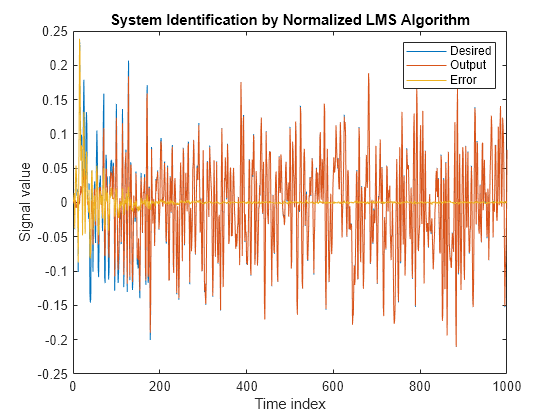
The output y of the adaptive filter is the signal converged to the desired signal d thereby minimizing the error e between the two signals.
plot(1:1000, [d,y,e])
title('System Identification by Normalized LMS Algorithm')
legend('Desired','Output','Error')
xlabel('Time index')
ylabel('Signal value')
Compare the Adapted Filter to the Unknown System
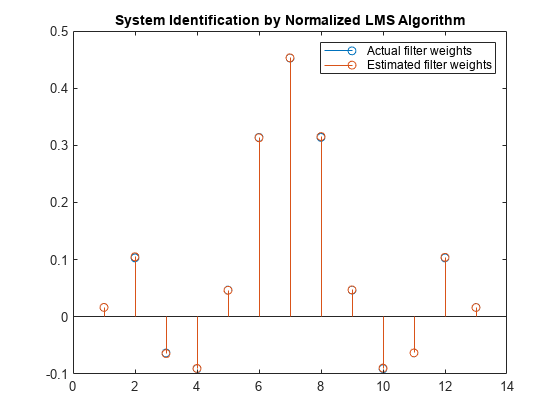
The weights vector w represents the coefficients of the LMS filter that is adapted to resemble the unknown system (FIR filter). To confirm the convergence, compare the numerator of the FIR filter and the estimated weights of the adaptive filter.
stem([(filt.Numerator).' w])
title('System Identification by Normalized LMS Algorithm')
legend('Actual filter weights','Estimated filter weights',...
       'Location','NorthEast')
See Also
Objects
Topics
- System Identification of FIR Filter Using LMS Algorithm
- Compare Convergence Performance Between LMS Algorithm and Normalized LMS Algorithm
References
[1] Hayes, Monson H., Statistical Digital Signal Processing and Modeling. Hoboken, NJ: John Wiley & Sons, 1996, pp.493–552.
[2] Haykin, Simon, Adaptive Filter Theory. Upper Saddle River, NJ: Prentice-Hall, Inc., 1996.