Gigasamples-per-Second Correlator and Peak Detector
This example shows how to implement a high-throughput frame-based correlator and peak detector. The system is suitable for applications such as lidar and mm-wave radar.
Lidar and radar systems operate by transmitting pulses, receiving the sent pulse in a stream of data, and using signal processing techniques to determine where in the receiver stream the pulse is located. When you design such a system, one of the main considerations is the pulse width or pulse duration. Pulse width is a measure (in seconds) of how long each pulse transmission is. Longer pulses have more energy and can therefore increase the range of the system. Shorter pulses cannot travel as far, but they can achieve greater accuracy in resolving the distance between objects. The pulse width determines the signal bandwidth. For example, a pulse width of 2 ns results in a signal bandwidth of 500 MS/s. The signal bandwidth is then used to determine the minimum distance where separate objects can be resolved from one another. This distance is the range ambiguity and is equal to c/(2*B), where c is the speed of light, and B is the signal bandwidth.
In high-precision lidar systems, the pulse width can often be as short as 4 ns. This width corresponds to a signal bandwidth of 250 MS/s and range ambiguity of 0.6 m. This calculation does not assume any additional signal processing, such as pulse compression, which could improve the accuracy. To meet the Nyquist rate, the received signal must be sampled at a rate of at least 500 MS/s. In practice, systems often oversample to improve performance. Typically, FPGAs run at up to 500 MHz. To process data with sample rates greater than the maximum clock rate, designs use frame-based processing, where each block operates on a vector of input data every clock cycle. In this way, the processing is parallel and sample rate is higher without an increase in clock rate. These designs can achieve gigasamples-per-second (GSPS) data rates, also called super sample rates.
This example describes a correlation and peak detection system that uses a 250 MHz clock and an input frame of 16 samples. These parameters enable the system to process a 4 GS/s input stream oversampled by a factor of 16.
Waveform Generation and Matched Filter Design
Broadly, lidar and radar systems can be split into pulsed waveform systems and continuous waveform systems. Pulsed waveform systems transmit bursts of data and then wait for a period, whereas continuous waveform systems are always transmitting. In each kind of system, you can apply different kinds of modulation to the waveform to enhance different properties such as range and resolution. This example shows a pulsed laser lidar system without signal modulation.
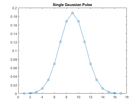
An ideal pulse has a rectangular shape in the time domain, corresponding to a sinc function in the frequency domain. The physical properties of laser systems mean that there is a ramp-up period to peak output, followed by a ramp-down period. Model this input by using a Gaussian function, then generate a stream of zeros and place pulses in the stream.
bt = 1; % 3 dB bandwidth-symbol time
sps = 16; % 16 times oversampled
span = 1; % 1 symbol
pulse = gaussdesign(bt,span,sps); % Pulse shape
plot(pulse,'o-');
title('Single Gaussian Pulse')
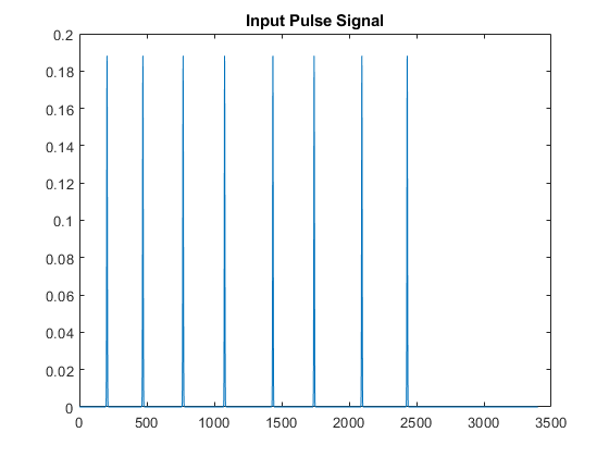
pulseLength = 17; % Number of samples per symbol
N = pulseLength * 200;  % 200 symbols
tx = zeros(N,1);
temp = primes(round(.80*N)); % Place pulses at a few scattered locations. Offset is a prime number.
locations = temp(45:45:end);
for index = 1:length(locations)
    tx(locations(index):locations(index) + pulseLength - 1) = pulse;
end
figure
plot(tx);
title('Input Pulse Signal')
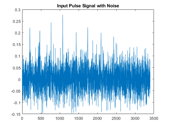
Now, add noise to simulate the channel and design a matched filter, which is the time-reversed conjugate of the pulse. Measure the noise inserted to make sure the calculation was correct. The pulse is symmetric and equivalent to the matched filter.
snr = 3;
pulseStream = awgn(tx,snr,10*log10(cov(pulse)),1);  % Add in AWGN.
figure
plot(pulseStream);
title('Input Pulse Signal with Noise')
noise = pulseStream - tx;
fprintf('Computed SNR is %3.2f \n',10*log10(cov(pulse)/cov(noise)));
h = flipud(conj(pulse));
isequal(h,pulse)
Computed SNR is 2.82

ans =

  logical

   1
Simulink Design
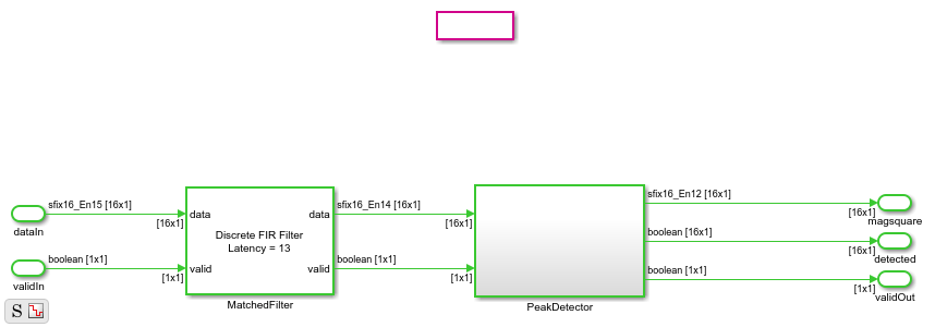
The example model implements a frame-based correlator and peak detector, using the input waveform and filter coefficients from the previous section. The CorrelatorPeakDetector subsystem has three outputs. The magnitude-squared matched filter output shows the boost in the signal-to-noise ratio (SNR) from the correlator. The detected output is a stream of Boolean values, which indicates when a pulse is detected. The valid output indicates when the output data is available.
vectorSize = 16;
windowLength = 19;
model = 'CorrelationandPeakDetection';
load_system(model)
set_param(model,'SimulationCommand','Update')
open_system(model)
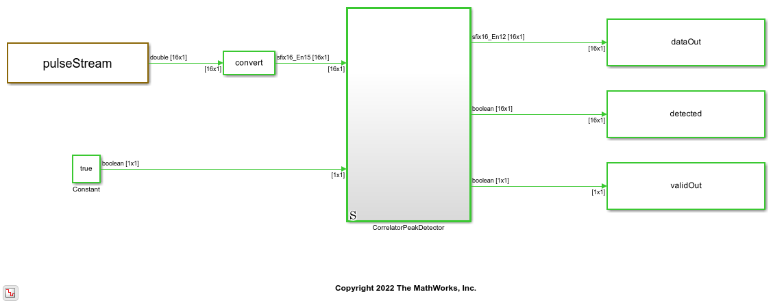
The DUT consists of a correlator or matched filter implemented using a Discrete FIR Filter block and a PeakDetector subsystem. The Discrete FIR Filter convolutes the input stream with the matched filter coefficients and passes the result to the PeakDetector subsystem. The PeakDetector uses a windowing method to determine local maxima.
model = 'CorrelationandPeakDetection/CorrelatorPeakDetector';
open_system(model)
The PeakDetector subsystem forms a sliding window of the FIR results, which is [19x1] for each element of the [16x1] input. An overall vector of [34x1] forms each subwindow. Inside the VectorPeakPick subsystem, the VectorTappedDelay subsystem forms this window and passes it to the subtract_midpoint subsystem, which implements the peak detection algorithm. The peak detection algorithm assumes that peaks are present when all values in the window subtracted by the middle value are less than or equal to 0. A For Each subsystem repeats this calculation 16 times to check each subwindow.
model = 'CorrelationandPeakDetection/CorrelatorPeakDetector/PeakDetector';
open_system(model)

Verification
Next, run the simulation and verify that the model detects pulses where you expect them, using the information from waveform generation.
sim('CorrelationandPeakDetection.slx')
xlocations = find(detected==1); % Find locations where peaks were detected.
prevxlocation = 0; % Check for multiple points for the same peak in the loop below.
addr = 1;
locationsHDL = zeros(length(locations),1);
for ii = 1:1:length(xlocations)  % If there are multiple points for the same peak, pick one.
    if xlocations(ii) ~= prevxlocation+1
        locationsHDL(addr) = xlocations(ii);
        addr = addr + 1;
        prevxlocation = xlocations(ii);
    end
end
latencyHDL = round(mean(locationsHDL - locations')); % Latency is constant, and is the difference between samples.
locationsDetected = locationsHDL - latencyHDL
locationsDetected =

         196
         463
         761
        1069
        1427
        1733
        2087
        2423
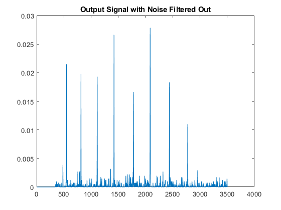
Observe the magnitude squared output to see that the matched filter has significantly boosted the SNR.
plot(dataOut);
title('Output Signal with Noise Filtered Out')
HDL Implementation Results
To generate HDL code from this example model, you must have the HDL Coder™ product. HDL was generated for the CorrelatorPeakDetector subsystem and synthesized with Xilinx® Vivado™ targeting a Xilinx Zynq®-7000 SoC ZC706 evaluation board. The design meets timing with a constraint of 400 MHz. The table shows the post place-and-route resource utilization results.
T = table(...
    categorical({'DSP';'LUT';'Flip Flop';'BRAM'}), ...
    categorical({'288'; '9549'; '9092';'0'}), ...
    'VariableNames',{'Resource','Usage'})
T =

  4×2 table

    Resource     Usage
    _________    _____

    DSP          288
    LUT          9549
    Flip Flop    9092
    BRAM         0
Sample Rate Modification Using Scalar Processing
You can adapt the model to process input with different sample rates. For example, you can process an input with 25 MS/s oversampled by a factor of 10 and, therefore, with a throughput of 250 MS/s using scalar rather than frame-based input. DSP HDL Toolbox™ library blocks automatically switch between frame and scalar algorithms according to the dimension of the data at the input port. In this example, you can choose to process frame or scalar input by modifying a single parameter, vector_size. The model automatically determines the correct dimensions for frame or scalar input and processes the data accordingly.
vectorSize = 1; % Scalar processing
sim('CorrelationandPeakDetection.slx') % Run simulation.
xlocations = find(detected==1); % Find locations where peaks are detected.
prevxlocation = 0; % Check for multiple points for the same peak in the loop below.
addr = 1;
locationsHDL = zeros(length(locations),1);
for ii = 1:1:length(xlocations)  % If there are multiple points for same peak, pick one.
    if xlocations(ii) ~= prevxlocation + 1
        locationsHDL(addr) = xlocations(ii);
        addr = addr + 1;
        prevxlocation = xlocations(ii);
    end
end
latencyHDL = round(mean(locationsHDL-locations')); % Latency is constant, and is the difference between samples.
locationsDetected = locationsHDL-latencyHDL
locationsDetected =

         196
         463
         761
        1069
        1427
        1733
        2087
        2423