NFC Digital Downconverter

DDC Structure

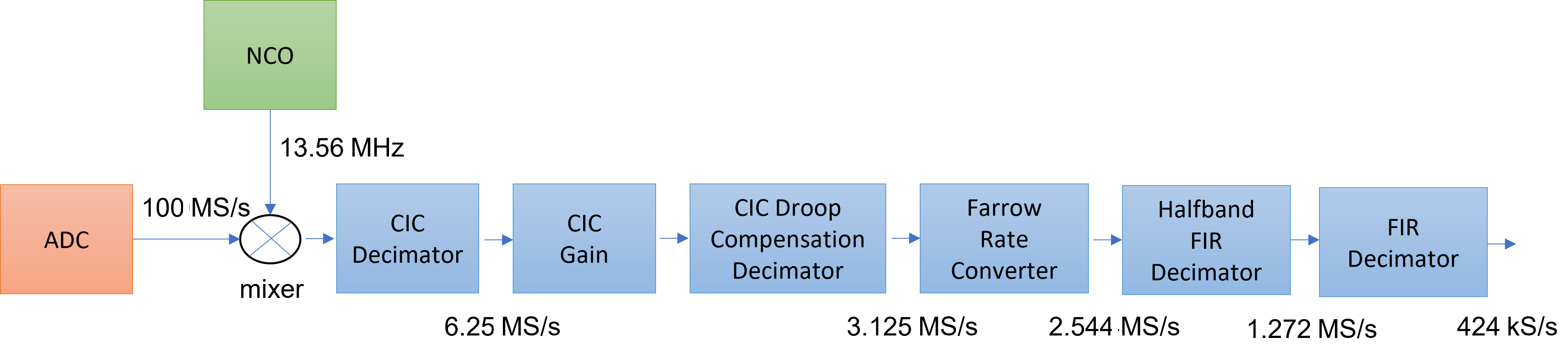
The DDC consists of a numerically controlled oscillator (NCO), mixer, and decimating filter chain. The filter chain consists of a cascade integrator-comb (CIC) decimator, CIC gain correction, CIC compensation decimator (FIR), Farrow rate converter, halfband FIR decimator, and a final FIR decimator.

The overall response of the filter chain is equivalent to that of a single decimation filter with the same specification. However, splitting the filter into multiple decimation stages results in a more efficient design that uses fewer hardware resources.

The CIC decimator provides a large initial decimation factor, which enables subsequent filters to work at lower rates. The CIC compensation decimator improves the spectral response by compensating for the CIC droop while decimating by two. The halfband is an intermediate decimator, and the final decimator implements the precise Fpass and Fstop characteristics of the DDC. The lower sampling rates near the end of the chain mean the later filters can optimize resource use by sharing multipliers.

This figure shows a block diagram of the DDC:

DDC Design

To design the DDC, you use floating-point operations and filter-design functions in MATLAB®.

DDC Parameters

This example designs the DDC filter characteristics to meet these specifications for the given input sampling rate and carrier frequency.

FsIn = 100e6;       % Sampling rate of DDC input
FsOut = 424e3;      % Sampling rate of DDC output
Fc = 13.56e6;       % Carrier frequency
Fpass = 424e3;      % Passband frequency, equivalent to sampling rate
Fstop = 480e3;      % Stopband frequency
Ap = 0.1;           % Passband ripple
Ast = 60;           % Stopband attenuation

CIC Decimator

The first filter stage is a CIC decimator because of its ability to efficiently implement a large decimation factor. The response of a CIC filter is similar to a cascade of moving average filters, but a CIC filter uses no multiplication or division. As a result, the CIC filter has a large DC gain.

cicParams.DecimationFactor = 16;
cicParams.DifferentialDelay = 1;
cicParams.NumSections = 3;
cicParams.FsOut = FsIn/cicParams.DecimationFactor;

cicFilt = dsp.CICDecimator(cicParams.DecimationFactor, ...
    cicParams.DifferentialDelay,cicParams.NumSections)
cicFilt.FixedPointDataType = 'Minimum section word lengths';
cicFilt.OutputWordLength = 18;
cicGain = gain(cicFilt)

cicFilt = 

  dsp.CICDecimator with properties:

      DecimationFactor: 16
     DifferentialDelay: 1
           NumSections: 3
    FixedPointDataType: 'Full precision'


cicGain =

        4096

Because the CIC gain is a power of two, a hardware implementation can easily correct for the gain factor by using a shift operation. For analysis purposes, the example represents the gain correction in MATLAB with a one-tap dsp.FIRFilter System object™.

cicGainCorr = dsp.FIRFilter('Numerator',1/cicGain)
cicGainCorr.FullPrecisionOverride = false;
cicGainCorr.CoefficientsDataType = 'Custom';
cicGainCorr.CustomCoefficientsDataType = numerictype(fi(cicGainCorr.Numerator,1,16));
cicGainCorr.OutputDataType = 'Custom';
cicGainCorr.CustomOutputDataType = numerictype(1,18,16);

cicGainCorr = 

  dsp.FIRFilter with properties:

            Structure: 'Direct form'
      NumeratorSource: 'Property'
            Numerator: 2.4414e-04
    InitialConditions: 0

  Use get to show all properties

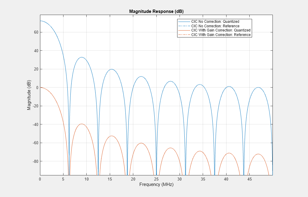
Display the magnitude response of the CIC filter with and without gain correction by using fvtool. For analysis, combine the CIC filter and the gain correction filter into a dsp.FilterCascade System object. CIC filters use fixed-point arithmetic internally, so fvtool plots both the quantized and unquantized responses.

ddcPlots.cicDecim = fvtool(...
    cicFilt, ...
    dsp.FilterCascade(cicFilt,cicGainCorr), ...
    'Fs',[FsIn,FsIn]);
legend(ddcPlots.cicDecim, ...
    'CIC No Correction', ...
    'CIC With Gain Correction');

CIC Droop Compensation Filter

Because the magnitude response of the CIC filter has a significant droop within the passband region, the example uses a FIR-based droop compensation filter to flatten the passband response. The droop compensator has the same properties as the CIC decimator. This filter implements decimation by a factor of two, so you must also specify bandlimiting characteristics for the filter. Use the design function to return a filter System object with the specified characteristics.

compParams.R = 2;                                % CIC compensation decimation factor
compParams.Fpass = Fstop;                        % CIC compensation passband frequency
compParams.FsOut = cicParams.FsOut/compParams.R; % New sampling rate
compParams.Fstop = compParams.FsOut - Fstop;     % CIC compensation stopband frequency
compParams.Ap = Ap;                              % Same passband ripple as overall filter
compParams.Ast = Ast;                            % Same stopband attenuation as overall filter

compSpec = fdesign.decimator(compParams.R,'ciccomp', ...
    cicParams.DifferentialDelay, ...
    cicParams.NumSections, ...
    cicParams.DecimationFactor, ...
    'Fp,Fst,Ap,Ast', ...
    compParams.Fpass,compParams.Fstop,compParams.Ap,compParams.Ast, ...
    cicParams.FsOut);
compFilt = design(compSpec,'SystemObject',true)


% Fixed point settings
compFilt.FullPrecisionOverride = false;
compFilt.CoefficientsDataType = 'Custom';
compFilt.CustomCoefficientsDataType = numerictype([],16,15);
compFilt.ProductDataType = 'Full precision';
compFilt.AccumulatorDataType = 'Full precision';
compFilt.OutputDataType = 'Custom';
compFilt.CustomOutputDataType = numerictype([],18,16);

compFilt = 

  dsp.FIRDecimator with properties:

   Main
    DecimationFactor: 2
     NumeratorSource: 'Property'
           Numerator: [-0.0282 -0.0462 0.1348 0.4382 0.4382 ... ] (1x8 double)
           Structure: 'Direct form'

  Use get to show all properties

Plot the response of the CIC droop compensation filter.

ddcPlots.cicComp = fvtool(compFilt, ...
    'Fs',FsIn,'Legend','off');

Farrow Rate Converter

Next, a Farrow filter converts the sampling rate into an integer multiple of the output sampling rate. This conversion means the remainder of the decimation filter chain can use integer decimation factors. To choose the output rate of this stage, consider an integer that you can factor easily into a few stages. The sample rate at the input to the Farrow rate converter is 3.125 MS/s, which is approximately a 7.3702 multiple of 424 kS/s (output rate). If the Farrow rate converter output rate was 7*424 kS/s, then the further decimation stages could not factor this rate into integer multiples. This example uses 6*424 kS/s as the output sampling rate of this stage. This rate change is approximately 1.22, and this decimation ratio has acceptable aliasing. Farrow filters with larger rate changes may have increased aliasing.

The default 3rd order LaGrange coefficients are derived from a closed-form solution and work for any rate change, so you do not need to design custom coefficients for this filter. The Farrow filter structure is the same as that used in the dsp.VariableIntegerDelay and dsp.FarrowRateConverter System objects.

These variables define the key parameters of the Farrow rate converter. FsIn and FsOut are the input and output rates, respectively.

farrowParams.FsIn = compParams.FsOut ;
farrowParams.FsOut = 6*424e3;
farrowParams.RateChange = farrowParams.FsIn/farrowParams.FsOut;
farrowFilt = dsp.FarrowRateConverter('InputSampleRate',farrowParams.FsIn, 'OutputSampleRate',farrowParams.FsOut);

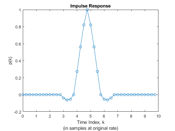
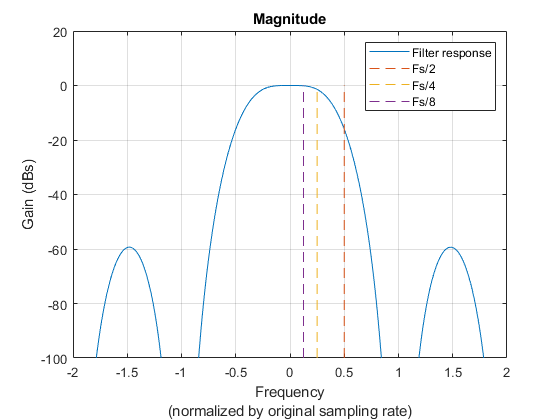
To evaluate the Farrow rate converter, generate an impulse input with a length of Lx samples. Then, calculate the oversampled impulse response of the Farrow-based variable fractional delay object. Pass the impulse response through the object at N different fractional delays from 0 through 1-(1/N). Store the results in the oversampled response vector p and plot the impulse and magnitude response.

Lx = 10;
x = zeros(Lx,1);
x(1) = 1;

vfd = dsp.VariableFractionalDelay( ...
    'InterpolationMethod','Farrow');

N = 4;
Lp = N * Lx;
p = zeros(Lp,1);


for n=1:N
    p(n:N:end) = vfd(x,4+(N-n)/N);
end

figure(1); clf;
t = (0:length(p)-1)/N;
plot(t,p,'-o');
title("Impulse Response");
xlabel("Time Index, k" + newline + "(in samples at original rate)");
ylabel("p(k)");

figure(2); clf;
Lfft = 1024;
Pmag = 20*log(abs(fft(p/N,1024)));
f = (0:Lfft-1) * N / Lfft;
plot(f-N/2,fftshift(Pmag)); hold on;
ax = axis;
plot([1/2 1/2],[ax(3) ax(4)],'--');
plot([1/4 1/4],[ax(3) ax(4)],'--');
plot([1/8 1/8],[ax(3) ax(4)],'--');
axis([ax(1) ax(2) -100 20]);
grid on;
title("Magnitude");
xlabel("Frequency" + newline + "(normalized by original sampling rate)");
ylabel("Gain (dBs)");
legend("Filter response","Fs/2","Fs/4","Fs/8");

Halfband Decimator

The halfband filter provides efficient decimation by two. Halfband filters are efficient because approximately half of their coefficients are equal to zero, and those multipliers are excluded from the hardware implementation.

hbParams.FsOut = farrowParams.FsOut/2;
hbParams.TransitionWidth = hbParams.FsOut - 2*Fstop;
hbParams.StopbandAttenuation = Ast;

hbSpec = fdesign.decimator(2,'halfband',...
    'Tw,Ast', ...
    hbParams.TransitionWidth, ...
    hbParams.StopbandAttenuation, ...
    farrowParams.FsOut);
hbFilt = design(hbSpec,'SystemObject',true)


% Fixed point settings
hbFilt.FullPrecisionOverride = false;
hbFilt.CoefficientsDataType = 'Custom';
hbFilt.CustomCoefficientsDataType = numerictype([],16,15);
hbFilt.ProductDataType = 'Full precision';
hbFilt.AccumulatorDataType = 'Full precision';
hbFilt.OutputDataType = 'Custom';
hbFilt.CustomOutputDataType = numerictype([],18,16);

hbFilt = 

  dsp.FIRDecimator with properties:

   Main
    DecimationFactor: 2
     NumeratorSource: 'Property'
           Numerator: [0.0020 0 -0.0054 0 0.0124 0 -0.0247 ... ] (1x27 double)
           Structure: 'Direct form'

  Use get to show all properties

Plot the response of the halfband filter output.

ddcPlots.halfbandFIR = fvtool(hbFilt, ...
    'Fs',FsIn,'Legend','off');

Final FIR Decimator

The final FIR implements the detailed passband and stopband characteristics of the DDC. This filter has more coefficients than the earlier FIR filters. However, because the filter operates at a lower sampling rate, it can use resource sharing for an efficient hardware implementation.

finalSpec = fdesign.decimator(2,'lowpass', ...
    'Fp,Fst,Ap,Ast',Fpass,Fstop,Ap,Ast,hbParams.FsOut);
finalFilt = design(finalSpec,'equiripple','SystemObject',true)


% Fixed point settings
finalFilt.FullPrecisionOverride = false;
finalFilt.CoefficientsDataType = 'Custom';
finalFilt.CustomCoefficientsDataType = numerictype([],16,15);
finalFilt.ProductDataType = 'Full precision';
finalFilt.AccumulatorDataType = 'Full precision';
finalFilt.OutputDataType = 'Custom';
finalFilt.CustomOutputDataType = numerictype([],18,16);

finalFilt = 

  dsp.FIRDecimator with properties:

   Main
    DecimationFactor: 2
     NumeratorSource: 'Property'
           Numerator: [-0.0024 -0.0012 0.0020 -0.0017 ... ] (1x63 double)
           Structure: 'Direct form'

  Use get to show all properties

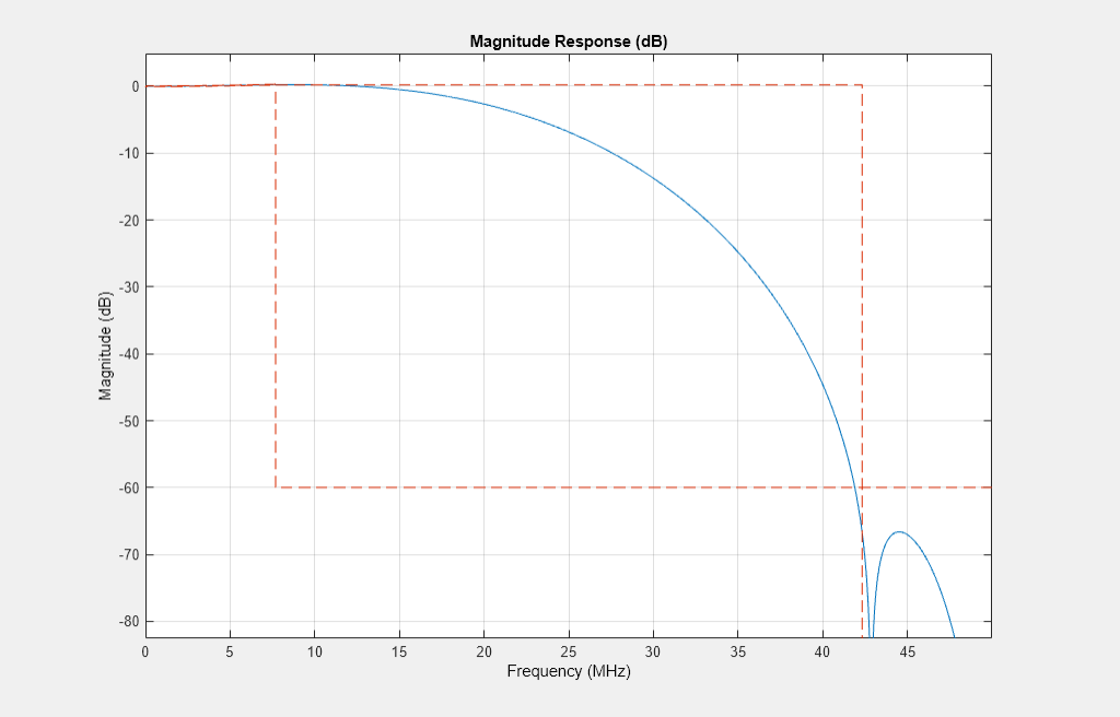
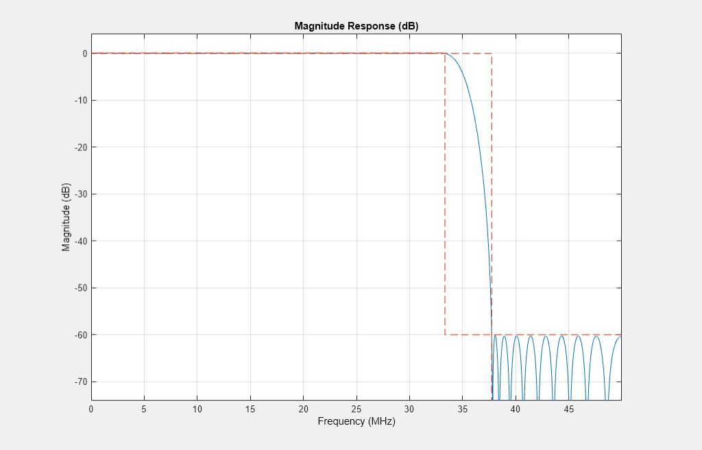
Visualize the magnitude response of the final FIR.

ddcPlots.overallResponse = fvtool(finalFilt,'Fs',FsIn,'Legend','off');

HDL-Optimized Simulink Model

The next step in the design flow is to implement the DDC in Simulink using blocks that support HDL code generation.

Model Configuration

The model relies on variables in the MATLAB workspace to configure the blocks and settings. It uses the same filter chain variables defined earlier in the example. Next, define the NCO characteristics and the input signal. The example uses these characteristics to configure the NCO block.

Specify the desired frequency resolution and calculate the number of accumulator bits that you need to achieve the desired resolution. Set the desired spurious free dynamic range, and then define the number of quantized accumulator bits. The NCO uses the quantized output of the accumulator to address the sine lookup table. Also, compute the phase increment that the NCO uses to generate the specified carrier frequency. The NCO applies phase dither to those accumulator bits that it removes during quantization.

nco.Fd = 1;
nco.AccWL = nextpow2(FsIn/nco.Fd)+1;
SFDR = 84;
nco.QuantAccWL = ceil((SFDR-12)/6);
nco.PhaseInc = round((-Fc*2^nco.AccWL)/FsIn);
nco.NumDitherBits = nco.AccWL-nco.QuantAccWL;

The input to the DDC comes from the ddcIn variable. For now, assign a dummy value for ddcIn so that the model can compute its data types. During testing, ddcIn provides input data to the model.

ddcIn = 0;

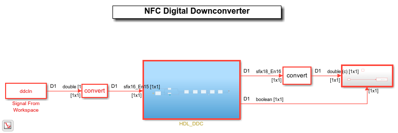
Model Structure

This figure shows the top level of the DDC Simulink model. The model imports the ddcIn variable from the MATLAB workspace by using a Signal From Workspace block, converts the input signal to 16-bit values, and applies the signal to the DDC. You can generate HDL code from the HDL_DDC subsystem.

modelName = 'DDCforNFCHDL';
 open_system(modelName);
 set_param(modelName,'SimulationCommand','Update');
 set_param(modelName,'Open','on');

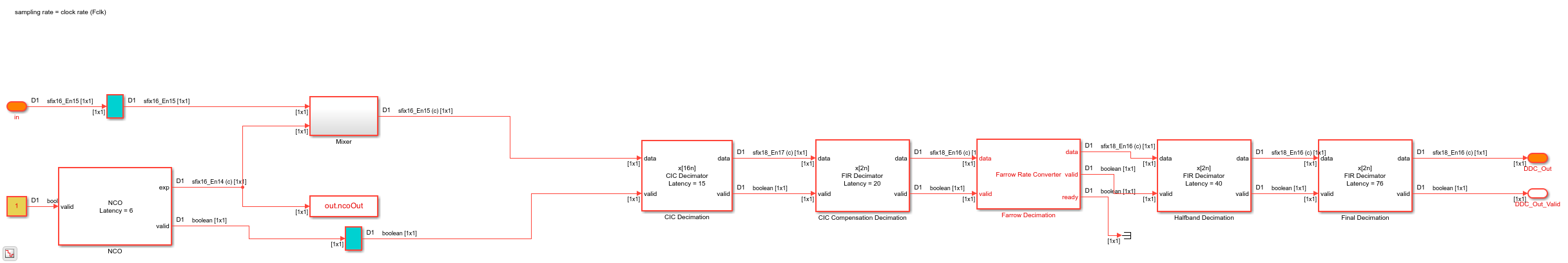
The HDL_DDC subsystem implements the DDC filter. First, the NCO block generates a complex phasor at the carrier frequency. This signal goes to a mixer that multiplies the phasor with the input signal. Then, the mixer passes the output to the filter chain, which decimates it to 424 kS/s.

set_param([modelName '/HDL_DDC'],'Open','on');

NCO Block Parameters

The NCO block in the model is configured with the parameters defined in the nco structure.

CIC Decimation and Gain Correction

The first filter stage is a CIC decimator that is implemented with a CIC Decimator block. The block parameters are set to the cicParams structure values. To implement the gain correction, the block has the Gain correction parameter selected.

The model configures the filters by using the properties of the corresponding System objects. The CIC compensation, halfband decimation, and final decimation filters operate at effective sample rates that are lower than the clock rate by factors of 16, 32, and 64, respectively. The model implements these sample rates by using the valid input signal to indicate which samples are valid at each rate. The signals in the filter chain all have the same Simulink sample time.

The CIC Compensation, Halfband Decimation, and Final Decimation filters are each implemented by an FIR Decimator. By setting the Minimum number of cycles between valid input samples parameter, you can use the invalid cycles between input samples to share resources. For example, the spacing between every input of CIC Compensation Decimator is 16.

The CIC Compensation Decimation, Halfband Decimation, and Final Decimation filters are fully serial and use one multiplier for the real parts of the samples and one multiplier for the imaginary parts. Each filter uses two multipliers in total. This resource saving is possible because of the large rate change. The Farrow Rate Converter uses one fully serial FIR filter (one multiplier) for each row of the coefficient matrix, for the real part of the samples and the imaginary part. The filter uses eight multipliers in total.

Sinusoid on Carrier Test and Verification

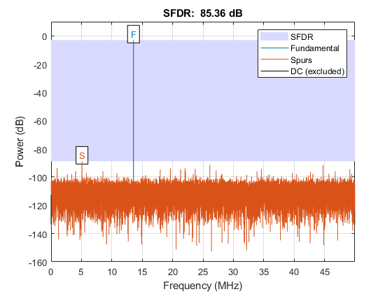
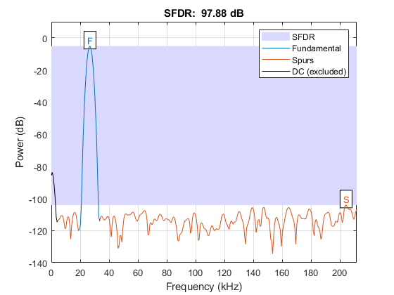
To test the DDC, modulate a 424 kHz sinusoid onto the carrier frequency and pass the modulated sine wave through the DDC. Then, measure the spurious-free dynamic range (SFDR) of the resulting tone and the SFDR of the NCO output. Plot the SFDR of the NCO and the fixed-point DDC output.

% Initialize random seed before executing any simulations.
rng(0);

% Generate a 40 kHz test tone, modulated onto the carrier.
ddcIn = DDCTestUtils.GenerateTestTone(40e3,Fc);

% Demodulate the test signal by running the Simulink model.
out = sim(modelName);

% Measure the SFDR of the NCO, floating-point DDC outputs, and fixed-point
% DDC outputs.
results.sfdrNCO = sfdr(real(out.ncoOut),FsIn);
results.sfdrFixedDDC = sfdr(real(out.ddcFixedOut),FsOut);

disp('SFDR Measurements');
disp(['   Fixed-point NCO SFDR: ',num2str(results.sfdrNCO) ' dB']);
disp(['   Optimized fixed-point DDC SFDR: ',num2str(results.sfdrFixedDDC) ' dB']);
fprintf(newline);

% Plot the SFDR of the NCO and fixed-point DDC outputs.
ddcPlots.ncoOutSDFR = figure;
sfdr(real(out.ncoOut),FsIn);

ddcPlots.OptddcOutSFDR = figure;
sfdr(real(out.ddcFixedOut),FsOut);

SFDR Measurements
   Fixed-point NCO SFDR: 85.3637 dB
   Optimized fixed-point DDC SFDR: 97.8753 dB

HDL Code Generation and FPGA Implementation

To generate the HDL code for this example, you must have the HDL Coder™ product. Use the makehdl and makehdltb commands to generate HDL code and an HDL test bench for the HDL_DDC subsystem. For this example, the DDC was synthesized on a Xilinx® Zynq®-7000 ZC706 evaluation board. The table shows the post place-and-route resource utilization results. The design met timing with a clock frequency of 340 MHz.

T = table(...
    categorical({'LUT'; 'LUTRAM'; 'FF'; 'BRAM'; 'DSP'}), ...
    categorical({'1547'; '386'; '3351'; '2'; '36'}), ...
    'VariableNames',{'Resource','Usage'})

T =

  5x2 table

    Resource    Usage
    ________    _____

     LUT        1547 
     LUTRAM     386  
     FF         3351 
     BRAM       2    
     DSP        36