Code Execution Profiling Report
You can configure a software-in-the-loop (SIL), processor-in-the-loop (PIL), or XCP-based
external mode simulation to produce execution-time metrics for generated code. The simulation
stores data in a workspace variable, for example, executionProfile. When
the simulation is complete, you can open a code execution profiling report by:
Using the Code Profile Analyzer. In the Results section, under Overall, click Generate Report.
Running
report(executionProfile)in the Command Window.
The report contains multiple sections.
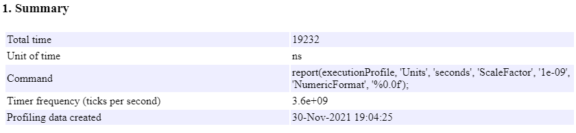
Summary
This section gives information about the creation of the report.
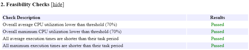
Feasibility Checks
If the number of timer ticks per second is known, the simulation performs feasibility checks and displays results in this section. The checks are shown in this table.
| Check | Comments |
|---|---|
| Overall average CPU utilization lower than threshold | The default threshold value is 70%. To change the threshold value, for example, to 85%, use this command: executionProfile.CPUUtilization=0.85; For information about CPU utilization, see section 5. |
| Overall maximum CPU utilization lower than threshold | |
| All average execution times are shorter than their task period | Use the results of these checks to verify that task overrun does not occur. |
| All maximum execution times are shorter than their task period |
Note
An external mode simulation does not produce this section.
In the Results column, the report displays Passed or Failed.
Profiled Sections of Code
This section contains information about profiled code sections. In the Section column, expand and collapse profiled sections by clicking [+] and [–] respectively. This graphic shows fully expanded sections.
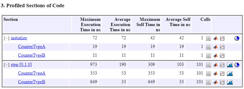
In this example, the report contains time measurements for:
The model initialization function
initialize.A task represented by the step function
step [0.1 0].Functions generated from the subsystems
CounterTypeAandCounterTypeB.
From the report, you can trace the model component that produces a set of metrics. For
example, in the Section column, if you click the
CounterTypeA hyperlink, the Simulink® Editor identifies the subsystem.

By default, the report displays time in nanoseconds (10-9 seconds). You can specify the time unit and numeric display format. For example, to display time in microseconds (10-6 seconds), use the following command:
report(executionProfile,...
         'Units', 'Seconds', ...
         'ScaleFactor', '1e-06', ...
         'NumericFormat', '%0.3f')
The report displays time in seconds only if the timer is calibrated, that is, the number of timer ticks per second is known. On a Windows® machine, the software determines this value for a SIL simulation. On a Linux® machine, calibrate the timer manually. For example, if your processor speed is 1 GHz, specify the number of timer ticks per second:
executionProfile.TimerTicksPerSecond = 1e9;
To view execution-time metrics for a task or function in the Command Window, on the
corresponding row, click ![]() .
.
>> executionProfile.Sections(5)
  ExecutionTimeCodeSection with properties:

                            Name: 'CounterTypeA'
                          Number: 5
            ExecutionTimeInTicks: [122 102 100 86 88 88 88 86 88 88 156 122  … ]
                 SelfTimeInTicks: [122 102 100 86 88 88 88 86 88 88 156 122  … ]
           TurnaroundTimeInTicks: [122 102 100 86 88 88 88 86 88 88 156 122  … ]
       TotalExecutionTimeInTicks: 19436
            TotalSelfTimeInTicks: 19436
      TotalTurnaroundTimeInTicks: 19436
     MaximumExecutionTimeInTicks: 1270
     MaximumExecutionTimeCallNum: 27
          MaximumSelfTimeInTicks: 1270
          MaximumSelfTimeCallNum: 27
    MaximumTurnaroundTimeInTicks: 1270
    MaximumTurnaroundTimeCallNum: 27
                        NumCalls: 101
          ExecutionTimeInSeconds: [3.3889e-08 2.8333e-08 2.7778e-08 2.3889e-08 … ]
                            Time: [101×1 double]
To display measured execution times in the Simulation Data Inspector, click the icon ![]() . Then, select the
. Then, select the step [0.1 0] and
CounterTypeB check boxes.
You can see how execution times for the step and child functions vary over simulation time.
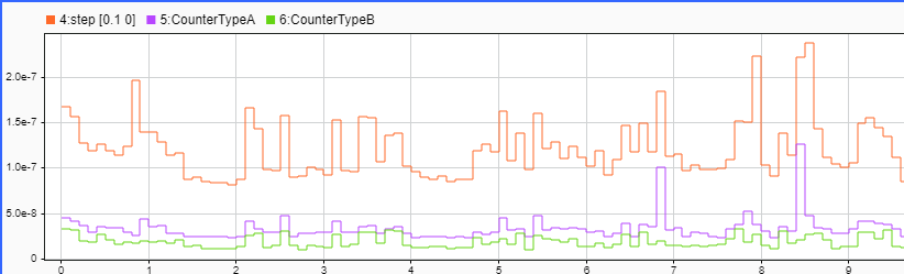
The execution time for the step function step [0 0.1] is
the sum of its self-time and execution times for the child functions
CounterTypeA and CounterTypeB. You can use the
Simulation Data Inspector to manage and compare plots from various simulations.
To display the execution-time distribution, click the icon ![]() .
.
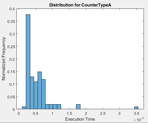
In this example, to create the histogram, the software uses these commands:
section=executionProfile.Sections(5);
data=section.ExecutionTimeInSeconds;
histogram(data, 30,'Normalization','probability');
If the generated code for your model contains nested functions, the simulation generates
pie charts that show the relative execution times of caller and called functions. To display
the pie charts, click the icon ![]() for the caller function. For example,
for the caller function. For example, step [0.1
0].
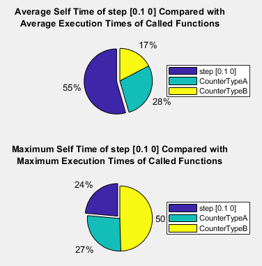
The pie charts can help you to identify functions that are bottlenecks in code execution.
This table describes the information that Profiled Sections of Code provides.
| Column | Description |
|---|---|
| Section | Name of task, top model, subsystem, or Model block. Click the link to go to the model. With a task, the sample period
and sample offset are listed next to the task name. For example, |
| Maximum Turnaround Time (Simulink Real-Time™ and support packages in real-time mode) | Longest time between start and end of code section. Includes preemption time. |
| Average Turnaround Time (Simulink Real-Time and support packages in real-time mode) | Average time between start and end of code section. Includes preemption time. |
| Maximum Execution Time | Longest time between start and end of code section. |
| Average Execution Time | Average time between start and end of code section. |
| Maximum Self Time | Maximum execution time, excluding time in child sections. |
| Average Self Time | Average execution time, excluding time in child sections. |
| Calls | Number of calls to the code section. |
Icon that you click to see the profiled code section in the Code view of the SIL/PIL app. The code section can be a task or a function. The specified workspace variable, for
example, | |
Icon that you click to display the profiled code section in the Command
Window. Equivalent to executing the command
The
specified workspace variable, for example, | |
Icon that you click to display measured execution times with Simulation Data Inspector. The specified workspace variable, for example,
| |
Icon that you click to display the execution-time distribution for the profiled code section. The specified workspace variable, for
example, | |
Icon that you click to display pie charts that show the relative execution times of caller and called functions in the generated code. |
Execution Times in Percentages
This section provides function execution times as percentages of caller function and total execution times, which can help you to identify performance bottlenecks in generated code.
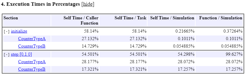
This table describes the information that each column provides.
| Column | Comparison Performed |
|---|---|
| Self Time / Caller Function | Function self time compared with the total execution time of the caller function. |
| Self Time / Task | Function self time compared with the total execution time of the task. |
| Self Time / Simulation | Function self time compared with the total execution time of the simulation. |
| Function / Simulation | Function execution time, which includes self time and time spent in child functions, compared with the total execution time of the simulation. |
Note
An external mode simulation does not produce this section.
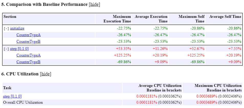
CPU Utilization
To help you to decide whether you can run the generated code on your target hardware, this section of the code execution profiling report provides CPU workload information:
Average and maximum CPU time required by each task during a sample period.
Total CPU usage in a sample period.
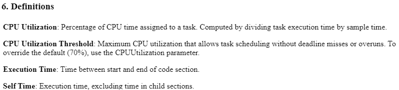
The software computes the percentage of CPU time assigned to a task by dividing task execution time by sample time.
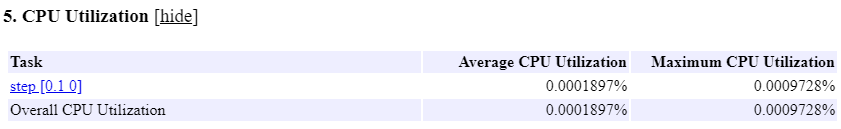
The software generates CPU Utilization only if the number of timer ticks per second is known.
Definitions
This section provides descriptions of some metrics.
Comparison with Baseline Performance
You can create a code execution profiling report that compares the performance of the
generated code against the performance of a reference version. For example, suppose you want
to use the execution-time metrics in executionProfile as the baseline for
SILTopModel.
In the Workspace panel, rename
executionProfiletoexecutionProfileBaseline.Run another SIL simulation.
To create a report that compares the latest performance against the baseline, in the Command Window, run:
report(executionProfile,'baseline', executionProfileBaseline)
In the report, the Comparison with Baseline Performance and CPU Utilization sections provide comparisons of execution-time metrics. The differences in execution-time metrics are color-coded:
Red — An increase in execution times or CPU usage.
Green — A decrease in execution times or CPU usage.
Black — No change.
Profiling Reports for Multiple Model Blocks
You can configure a top-model simulation that runs multiple Model blocks in SIL or PIL mode with code execution profiling enabled. When you run the simulation, it generates separate code execution profiling reports for the referenced models.
Open the top model that contains Model blocks. For example, at the command line, enter:
openExample('ecoder/SILPILVerificationExample', ...
             supportingFile='SILModelBlock.slx')
On the SIL/PIL tab, in the Mode section, specify SIL/PIL Simulation Only.
In the Prepare section, specify these settings:
System Under Test —
Model blocks in SIL/PIL
                    mode
Top Model Mode —
Normal
Model block
Counter Ais already configured to run in SIL mode. For Model blockCounter B, specify these parameters:Simulation mode —
Software-in-the-loop
                    (SIL)
Code interface —
Normal
Both Model blocks reference the model
SILCounter. To generate execution times for the Model blocks:Select
CounterAorCounterB.On the Model Block tab, in the Actions section, click Open as Top Model.
On the SIL/PIL tab, in the Settings gallery, click Functions to
COARSE, which sets the Measure function execution times configuration parameter forSILCountertoCoarse (referenced models and subsystems only).
To run a top-model simulation:
Select the
SILModelBlockwindow.On the SIL/PIL tab, in the Run section, click Run SIL/PIL.
Since the Single simulation output check box is selected, the simulation creates the variable
executionProfileinout, aSimulink.SimulationOutputobject.When the simulation is complete, to show the number of Model blocks that are profiled, in the Command Window, enter:
NumOfReports=out.executionProfile.getModuleNumber()
NumOfReports =
     2
To open the report for
CounterA, the first Model block, run:report(out.executionProfile.getModule(1))
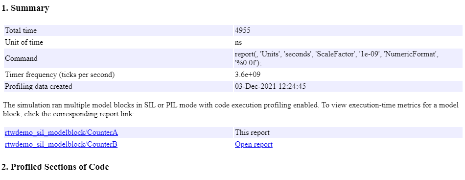
In the Summary section, the report provides a link to the second Model block report. To open the report for
CounterB, click Open report or run:report(out.executionProfile.getModule(2))
For more information about generating function execution times for model reference hierarchies, see Control Profiling Granularity.