Assess Stationarity of a Time Series
This example shows how to check whether a linear time series is a unit root process in several ways. You can assess unit root nonstationarity statistically, visually, and algebraically.
Simulate Data
Suppose that the true model for a linear time series is

where the innovation series  is iid with mean 0 and variance 1.5. Simulate data from this model. This model is a unit root process because the lag polynomial of the right side has characteristic root 1.
Mdl = arima('AR',0.2,'MA',-0.5,'D',1,'Constant',0,...
'Variance',1.5);
T = 30;
rng(5);
Y = simulate(Mdl,T);
Assess Stationarity Statistically
Econometrics Toolbox™ has four formal tests to choose from to check if a time series is nonstationary: adftest, kpsstest, pptest, and vratiotest. Use adftest to perform the Dickey-Fuller test on the data that you simulated in the previous steps.
adftest(Y)
ans =

  logical

   0
The test result indicates that you should not reject the null hypothesis that the series is a unit root process.
Assess Stationarity Visually
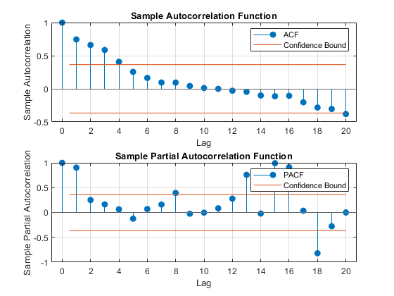
Suppose you don't have the time series model, but you have the data. Inspect a plot of the data. Also, inspect the plots of the sample autocorrelation function (ACF) and sample partial autocorrelation function (PACF).
plot(Y);
title('Simulated Time Series')
xlabel('t')
ylabel('Y')

subplot(2,1,1)
autocorr(Y)
subplot(2,1,2)
parcorr(Y)

The downward sloping of the plot indicates a unit root process. The lengths of the line segments on the ACF plot gradually decay, and continue this pattern for increasing lags. This behavior indicates a nonstationary series.
Assess Stationarity Algebraically
Suppose you have the model in standard form:

Write the equation in lag operator notation and solve for  to get

Use LagOp to convert the rational polynomial to a polynomial. Also, use isStable to inspect the characteristic roots of the denominator.
num = LagOp([1 -0.5]);
denom = LagOp([1 -1.2 0.2]);
quot = mrdivide(num,denom);

[r1,r2] = isStable(denom)
Warning: Termination window not currently open and coefficients
         are not below tolerance.

r1 =

  logical

   0


r2 =

    1.0000
    0.2000
This warning indicates that the resulting quotient has a degree larger than 1001, e.g., there might not be a terminating degree. This indicates instability. r1 = 0 indicates that the denominator is unstable. r2 is a vector of characteristics roots, one of the roots is 1. Therefore, this is a unit root process.
isStable is a numerical routine that calculates the characteristic values of a polynomial. If you use quot as an argument to isStable, then the output might indicate that the polynomial is stable (i.e., all characteristic values are slightly less than 1). You might need to adjust the tolerance options of isStable to get more accurate results.