Change the Bandwidth of a HAC Estimator

Open Live Script

This example shows how to change the bandwidth when estimating a HAC coefficient covariance, and compare estimates over varying bandwidths and kernels.

How does the bandwidth affect HAC estimators? If you change it, are there large differences in the estimates, and, if so, are the differences practically significant? Explore bandwidth effects by estimating HAC coefficient covariances over a grid of bandwidths.

Load and Plot Data

Determine how the cost of living affects the behavior of nominal wages. Load the Nelson Plosser data set to explore their statistical relationship.

load Data_NelsonPlosser
DTT = rmmissing(DataTimeTable);
cpi = DTT.CPI;            % Cost of living
wm = DTT.WN;              % Nominal wages

figure
plot(DTT.CPI,DTT.WN,"o")
hFit = lsline;  % Regression line
xlabel("Consumer Price Index (1967 = 100)")
ylabel("Nominal Wages (current $)")
legend(hFit,"OLS Line",Location="southeast")
title("{\bf Cost of Living}")
grid on

Figure contains an axes object. The axes object with title blank Cost blank of blank Living, xlabel Consumer Price Index (1967 = 100), ylabel Nominal Wages (current $) contains 2 objects of type line. One or more of the lines displays its values using only markers This object represents OLS Line.

The plot suggests that a linear model might capture the relationship between the two variables.

Define Model

Model the behavior of nominal wages with respect to CPI as this linear model.

${wm}_{t} = β_{0} + β_{1} {cpi}_{t} + ε_{t}$

Mdl = fitlm(DTT.CPI,DTT.WN)

Mdl = 
Linear regression model:
    y ~ 1 + x1

Estimated Coefficients:
                   Estimate      SE       tStat      pValue  
                   ________    ______    _______    _________

    (Intercept)    -2541.5     174.64    -14.553    2.407e-21
    x1              88.041     2.6784     32.871    4.507e-40


Number of observations: 62, Error degrees of freedom: 60
Root Mean Squared Error: 494
R-squared: 0.947,  Adjusted R-Squared: 0.947
F-statistic vs. constant model: 1.08e+03, p-value = 4.51e-40

coeffCPI = Mdl.Coefficients.Estimate(2);
seCPI = Mdl.Coefficients.SE(2);

Plot Residuals

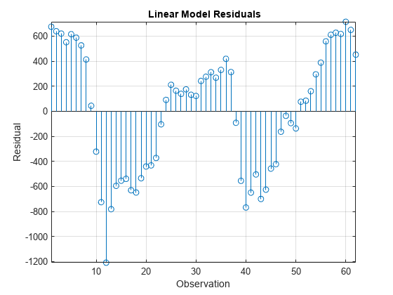
Plot the residuals from Mdl against the fitted values to assess heteroscedasticity and autocorrelation.

figure
stem(Mdl.Residuals.Raw)
xlabel("Observation")
ylabel("Residual")
title("{\bf Linear Model Residuals}")
axis tight
grid on

Figure contains an axes object. The axes object with title blank Linear blank Model blank Residuals, xlabel Observation, ylabel Residual contains an object of type stem.

The residual plot shows varying levels of dispersion, which indicates heteroscedasticity. Neighboring residuals (with respect to observation) tend to have the same sign and magnitude, which indicates the presence of autocorrelation.

Estimate HAC standard errors.

Obtain HAC standard errors over varying bandwidths using the Bartlett (for the Newey-West estimate) and quadratic spectral kernels.

numEstimates = 10;
stdErrBT = zeros(numEstimates,1);
stdErrQS = zeros(numEstimates,1);

for bw = 1:numEstimates
    [~,CoeffTbl] = hac(DTT,ResponseVariable="WN",PredictorVariables="CPI", ...
        Bandwidth=bw,Display="off");    % Newey-West
    [~,CoeffTblQS] = hac(DTT,ResponseVariable="WN",PredictorVariables="CPI", ...
        Weights="QS",Bandwidth=bw,Display="off");   % HAC using quadratic spectral kernel
    stdErrBT(bw) = CoeffTbl.SE(2);
    stdErrQS(bw) = CoeffTblQS.SE(2);
end

You can increase numEstimates to discover how increasing bandwidths affect the HAC estimates.

Plot Standard Errors

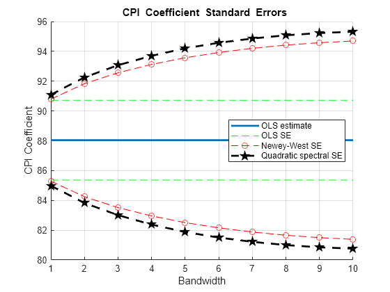
Visually compare the Newey-West standard errors of ${β_{}^{ˆ}}_{1}$ to those using the quadratic spectral kernel over the bandwidth grid.

figure
hold on
hCoeff = plot(1:numEstimates,repmat(coeffCPI,numEstimates,1), ...
    LineWidth=2);
hOLS = plot(1:numEstimates,repmat(coeffCPI+seCPI,numEstimates,1), ...
    "g--");
plot(1:numEstimates,repmat(coeffCPI-seCPI,numEstimates,1),"g--")
hBT = plot(1:numEstimates,coeffCPI+stdErrBT,"ro--");
plot(1:numEstimates,coeffCPI-stdErrBT,"ro--")
hQS = plot(1:numEstimates,coeffCPI+stdErrQS,"kp--", ...
    LineWidth=2);
plot(1:numEstimates,coeffCPI-stdErrQS,"kp--",LineWidth=2)
hold off
xlabel("Bandwidth")
ylabel("CPI Coefficient")
legend([hCoeff,hOLS,hBT,hQS],["OLS estimate" "OLS SE" ...
    "Newey-West SE" "Quadratic spectral SE"],Location="east")
title("{\bf CPI Coefficient Standard Errors}")
grid on

Figure contains an axes object. The axes object with title blank CPI blank Coefficient blank Standard blank Errors, xlabel Bandwidth, ylabel CPI Coefficient contains 7 objects of type line. These objects represent OLS estimate, OLS SE, Newey-West SE, Quadratic spectral SE.

The plot suggests that, for this data set, accounting for heteroscedasticity and autocorrelation using either HAC estimate results in more conservative intervals than the usual OLS standard error. The precision of the HAC estimates decreases as the bandwidth increases along the defined grid.

For this data set, the Newey-West estimates are slightly more precise than those using the quadratic spectral kernel. This might be because the latter captures heteroscedasticity and autocorrelation better than the former.

References:

Andrews, D. W. K. "Heteroskedasticity and Autocorrelation Consistent Covariance Matrix Estimation." Econometrica. Vol. 59, 1991, pp. 817-858.
Newey, W. K., and K. D. West. "A Simple, Positive Semi-definite, Heteroskedasticity and Autocorrelation Consistent Covariance Matrix." Econometrica. Vol. 55, No. 3, 1987, pp. 703-708.\
Newey, W. K., and K. D. West. "Automatic Lag Selection in Covariance Matrix Estimation." The Review of Economic Studies. Vol. 61, No. 4, 1994, pp. 631-653.

Related Examples

More About

Nonspherical Models