Choose Lags for ARMA Error Model

This example shows how to use Akaike Information Criterion (AIC) to select the nonseasonal autoregressive and moving average lag polynomial degrees for a regression model with ARMA errors.

Estimate several models by passing the data to estimate. Vary the autoregressive and moving average degrees p and q, respectively. Each fitted model contains an optimized loglikelihood objective function value, which you pass to aicbic to calculate AIC fit statistics. The AIC fit statistic penalizes the optimized loglikelihood function for complexity (i.e., for having more parameters).

Simulate response and predictor data for the regression model with ARMA errors:

where $${\epsilon }_t$$ is Gaussian with mean 0 and variance 1.

Mdl0 = regARIMA('Intercept',2,'Beta',[-2; 1.5],...
    'AR',{0.75, -0.5},'MA',0.7,'Variance',1); 

rng(2);            % For reproducibility
X = randn(1000,2); % Predictors
y = simulate(Mdl0,1000,'X',X);

Regress the response onto the predictors. Plot the residuals (i.e., estimated unconditional disturbances).

Fit = fitlm(X,y);
u = Fit.Residuals.Raw;

figure
plot(u)
title('{\bf Estimated Unconditional Disturbances}')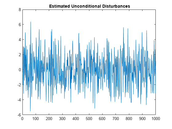

Plot the ACF and PACF of the residuals.

figure
subplot(2,1,1)
autocorr(u)
subplot(2,1,2)
parcorr(u)

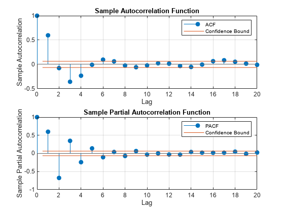
The ACF and PACF decay slowly, which indicates an ARMA process. It is difficult to use these correlograms to determine the lags. However, it seems reasonable that both polynomials should have four or fewer lags based on the lengths of the autocorrelations and partial autocorrelations.

To determine the number of AR and MA lags, define and estimate regression models with ARMA(p, q) errors by varying p = 1,..,3 and q = 1,...,3. Store the optimized loglikelihood objective function value for each model fit.

pMax = 3;
qMax = 3;
LogL = zeros(pMax,qMax);
SumPQ = LogL;

for p = 1:pMax
    for q = 1:qMax
        Mdl = regARIMA(p,0,q);
        [~,~,LogL(p,q)] = estimate(Mdl,y,'X',X,...
            'Display','off');
        SumPQ(p,q) = p+q;
    end
end

Calculate AIC for each model fit. The number of parameters is p + q + 4 (i.e., the intercept, two regression coefficients, and innovation variance).

logL = reshape(LogL,pMax*qMax,1);...
    % Elements taken column-wise 
numParams = reshape(SumPQ,pMax*qMax,1) + 4;
aic = aicbic(logL,numParams);
AIC = reshape(aic,pMax,qMax)

AIC = 3×3
103 ×

    3.1323    3.0195    2.9984
    2.9280    2.9297    2.9314
    2.9297    2.9305    2.9321

minAIC = min(aic)

minAIC = 
2.9280e+03

[bestP,bestQ] = find(AIC == minAIC)

bestP = 
2

bestQ = 
1

The best fitting model is the regression model with AR(2,1) errors because its corresponding AIC is the lowest.

See Also

aicbic | estimate

Related Examples

• Estimate Regression Model with ARIMA Errors

More About

• Select Regression Model with ARIMA Errors