Forecast a Regression Model with ARIMA Errors

This example shows how to forecast a regression model with ARIMA(3,1,2) errors using forecast and simulate.

Simulate two Gaussian predictor series with mean 2 and variance 1.

rng(1);
T = 50; % Sample size
X = randn(T,2) + 2;

Specify the regression model with ARIMA(3,1,2) errors:

where $${\epsilon }_t$$ is Gaussian with mean 0 and variance 2.

Mdl = regARIMA('Intercept',3,'Beta',[-2;1.5],'AR',{0.9,-0.5,0.2},...
    'D',1','MA',{0.75,-0.15},'Variance',2);

Mdl is a fully specified regression model with ARIMA(3,1,2) errors. Methods such as simulate and forecast require a fully specified model.

Simulate 30 observations from Mdl.

[y,e,u] = simulate(Mdl,30,'X',X(1:30,:));

y contains the simulated responses. e and u contain the corresponding simulated innovations and unconditional disturbances, respectively. It is best practice to provide forecast with presample innovations and unconditional disturbances if they are available.

Compute MMSE forecasts for Mdl 20 periods into the future using forecast. Compute the corresponding 95% forecast intervals.

[yF,yMSE] = forecast(Mdl,20,'X0',X(1:30,:),'U0',u,...
    'E0',e,'XF',X(31:T,:));
yFCI = [yF,yF] + 1.96*[-sqrt(yMSE),sqrt(yMSE)];

yFCI is a 20-by-2 matrix containing the 20 forecast intervals. The first column of yFCI contains the lower bounds for the forecast intervals, and the second column contains the upper bounds.

Forecast Mdl 20 periods into the future using Monte Carlo simulation. Compute the corresponding 95% forecast intervals

yMC = simulate(Mdl,20,'numPaths',1000,'X',X(31:T,:),'U0',u,'E0',e);
yMCBar = mean(yMC,2);
yMCCI = prctile(yMC,[2.5,97.5],2);

yMCBar is a 20-by-1 vector that contains the Monte Carlo forecasts over the forecast horizon. Like yFCI, yMMCI is a 20-by-2 matrix containing the forecast intervals, but based on the Monte Carlo simulation.

Plot the two forecast sets and their corresponding 95% forecast intervals.

figure
h1 = plot(1:30,y);
title('{\bf Forecasts and 95% Forecast Intervals}')
hold on
h2 = plot(31:50,yF,'r','LineWidth',2);
h3 = plot(31:50,yFCI,'r--','LineWidth',2);
h4 = plot(31:50,yMCBar,'k','LineWidth',2);
h5 = plot(31:50,yMCCI,'k--','LineWidth',2);
plot(30:31,[repmat(y(end),3,1),[yF(1),yFCI(1,:)]'],'b')
legend([h1,h2,h3(1),h4,h5(1)],'Observations','MMSE Forecasts',...
    'MMSE Forecast Intervals','Monte Carlo Forecasts',...
    'Monte Carlo Forecast Intervasls','Location','SouthWest')
xlabel('Time')
ylabel('y')
axis tight
hold off

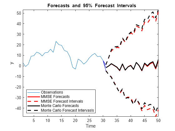
The MMSE and Monte Carlo forecasts are virtually equivalent. There are minor discrepancies between the forecast intervals.

The width of the forecast intervals increases as time increases. This is a consequence of forecasting with integrated errors.

See Also

regARIMA | estimate | forecast

Related Examples

• Forecast a Regression Model with Multiplicative Seasonal ARIMA Errors
• Verify Predictive Ability Robustness of a regARIMA Model

More About

• MMSE Forecasting Regression Models with ARIMA Errors
• Monte Carlo Forecasting of regARIMA Models