Information Criteria for Model Selection

Misspecification tests, such as the likelihood ratio (lratiotest), Lagrange multiplier (lmtest), and Wald (waldtest) tests, are appropriate only for comparing nested models. In contrast, information criteria are model selection tools to compare any models fit to the same data—the models being compared do not need to be nested.

Information criteria are likelihood-based measures of model fit that include a penalty for complexity (specifically, the number of parameters). Different information criteria are distinguished by the form of the penalty, and can favor different models.

Let $\log L (\hat{θ})$ denote the value of the maximized loglikelihood objective function for a model with k parameters fit to T data points. The aicbic function returns these information criteria:

Akaike information criterion (AIC). — The AIC compares models from the perspective of information entropy, as measured by Kullback-Leibler divergence. The AIC for a given model is

$- 2 \log L (\hat{θ}) + 2 k .$
Bayesian (Schwarz) information criterion (BIC) — The BIC compares models from the perspective of decision theory, as measured by expected loss. The BIC for a given model is

$- 2 \log L (\hat{θ}) + k \log (T) .$
Corrected AIC (AICc) — In small samples, AIC tends to overfit. The AICc adds a second-order bias-correction term to the AIC for better performance in small samples. The AICc for a given model is

$AIC + \frac{2 k (k + 1)}{T - k - 1} .$
The bias-correction term increases the penalty on the number of parameters relative to the AIC. Because the term approaches 0 with increasing sample size, AICc approaches AIC asymptotically.
The analysis in [3] suggests using AICc when numObs/numParam < 40.
Consistent AIC (CAIC) — The CAIC imposes an additional penalty for complex models, as compared to the BIC. The CAIC for a given model is

$- 2 \log L (\hat{θ}) + k (\log (T) + 1) = BIC + k .$
Hannan-Quinn criterion (HQC) — The HQC imposes a smaller penalty on complex models than the BIC in large samples. The HQC for a given model is

$- 2 \log L (\hat{θ}) + 2 k \log (\log (T)) .$

Regardless of the information criterion, when you compare values for multiple models, smaller values of the criterion indicate a better, more parsimonious fit.

Some experts scale information criteria values by T. aicbic scales results when you set the 'Normalize' name-value pair argument to true.

Compute Information Criteria Using `aicbic`

Open Live Script

This example shows how to use aicbic to compute information criteria for several competing GARCH models fit to simulated data. Although this example uses aicbic, some Statistics and Machine Learning Toolbox™ and Econometrics Toolbox™ model fitting functions also return information criteria in their estimation summaries.

Simulate Data

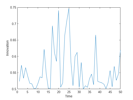
Simulate a random path of length 50 from the ARCH(1) data generating process (DGP)

$\begin{array}{rclrclrclrclrclrclrclrclrclrclrclrclrclrclrclrclrclrclrclrcl} y_{t} & = & ε_{t} \\ ε_{t}^{2} & = & 0.5 + 0.1 ε_{t - 1}^{2}, \end{array}$

where $ε_{t}$ is a random Gaussian series of innovations.

rng(1)  % For reproducibility
DGP = garch('ARCH',{0.1},'Constant',0.5);
T = 50;
y = simulate(DGP,T);

plot(y)
ylabel('Innovation')
xlabel('Time')

Figure contains an axes object. The axes object with xlabel Time, ylabel Innovation contains an object of type line.

Create Competing Models

Assume that the DGP is unknown, and that the ARCH(1), GARCH(1,1), ARCH(2), and GARCH(1,2) models are appropriate for describing the DGP.

For each competing model, create a garch model template for estimation.

Mdl(1) = garch(0,1);
Mdl(2) = garch(1,1);
Mdl(3) = garch(0,2);
Mdl(4) = garch(1,2);

Estimate Models

Fit each model to the simulated data y, compute the loglikelihood, and suppress the estimation display.

numMdl = numel(Mdl);
logL = zeros(numMdl,1);      % Preallocate
numParam = zeros(numMdl,1);
for j = 1:numMdl
    [EstMdl,~,logL(j)] = estimate(Mdl(j),y,'Display','off');
    results = summarize(EstMdl);
    numParam(j) = results.NumEstimatedParameters;
end

Compute and Compare Information Criteria

For each model, compute all available information criteria. Normalize the results by the sample size T.

[~,~,ic] = aicbic(logL,numParam,T,'Normalize',true)

ic = struct with fields:
     aic: [1.7619 1.8016 1.8019 1.8416]
     bic: [1.8384 1.9163 1.9167 1.9946]
    aicc: [1.7670 1.8121 1.8124 1.8594]
    caic: [1.8784 1.9763 1.9767 2.0746]
     hqc: [1.7911 1.8453 1.8456 1.8999]

ic is a 1-D structure array with a field for each information criterion. Each field contains a vector of measurements; element j corresponds to the model yielding loglikelihood logL(j).

For each criterion, determine the model that yields the minimum value.

[~,minIdx] = structfun(@min,ic);
[Mdl(minIdx).Description]'

ans = 5x1 string
    "GARCH(0,1) Conditional Variance Model (Gaussian Distribution)"
    "GARCH(0,1) Conditional Variance Model (Gaussian Distribution)"
    "GARCH(0,1) Conditional Variance Model (Gaussian Distribution)"
    "GARCH(0,1) Conditional Variance Model (Gaussian Distribution)"
    "GARCH(0,1) Conditional Variance Model (Gaussian Distribution)"

The model that minimizes all criteria is the ARCH(1) model, which has the same structure as the DGP.

References

[1] Akaike, Hirotugu. "Information Theory and an Extension of the Maximum Likelihood Principle.” In Selected Papers of Hirotugu Akaike, edited by Emanuel Parzen, Kunio Tanabe, and Genshiro Kitagawa, 199–213. New York: Springer, 1998. https://doi.org/10.1007/978-1-4612-1694-0_15.

[2] Akaike, Hirotugu. “A New Look at the Statistical Model Identification.” IEEE Transactions on Automatic Control 19, no. 6 (December 1974): 716–23. https://doi.org/10.1109/TAC.1974.1100705.

[3] Burnham, Kenneth P., and David R. Anderson. Model Selection and Multimodel Inference: A Practical Information-Theoretic Approach. 2nd ed, New York: Springer, 2002.

[4] Hannan, Edward J., and Barry G. Quinn. “The Determination of the Order of an Autoregression.” Journal of the Royal Statistical Society: Series B (Methodological) 41, no. 2 (January 1979): 190–95. https://doi.org/10.1111/j.2517-6161.1979.tb01072.x.

[5] Lütkepohl, Helmut, and Markus Krätzig, editors. Applied Time Series Econometrics. 1st ed. Cambridge University Press, 2004. https://doi.org/10.1017/CBO9780511606885.

[6] Schwarz, Gideon. “Estimating the Dimension of a Model.” The Annals of Statistics 6, no. 2 (March 1978): 461–64. https://doi.org/10.1214/aos/1176344136.