Simulate a Regression Model with Nonstationary Errors

This example shows how to simulate responses from a regression model with ARIMA unconditional disturbances, assuming that the predictors are white noise sequences.

Specify the regression model with ARIMA errors:

where the innovations are Gaussian with variance 1.

T = 150; % Sample size
Mdl = regARIMA('MA',{1.4,0.8},'AR',0.5,'Intercept',3,...
    'Variance',1,'Beta',[2;-1.5],'D',1);

Simulate two Gaussian predictor series with mean 0 and variance 1.

rng(1); % For reproducibility
X = randn(T,2);

Simulate and plot the response series.

y = simulate(Mdl,T,'X',X);

figure;
plot(y);
title 'Simulated Responses';
axis tight;

Regress y onto X. Plot the residuals, and test them for a unit root.

RegMdl = fitlm(X,y);

figure;
subplot(2,1,1);
plotResiduals(RegMdl,'caseorder');
subplot(2,1,2);
plotResiduals(RegMdl,'lagged');

h = adftest(RegMdl.Residuals.Raw)

h = logical
   0

The residual plots indicate that they are autocorrelated and possibly nonstationary (as constructed). h = 0 indicates that there is insufficient evidence to suggest that the residual series is not a unit root process.

Treat the nonstationary unconditional disturbances by transforming the data appropriately. In this case, difference the responses and predictors. Reestimate the regression model using the transformed responses, and plot the residuals.

dY = diff(y);
dX = diff(X);
dRegMdl = fitlm(dX,dY);

figure;
subplot(2,1,1);
plotResiduals(dRegMdl,'caseorder','LineStyle','-');
subplot(2,1,2);
plotResiduals(dRegMdl,'lagged');

h = adftest(dRegMdl.Residuals.Raw)

h = logical
   1

The residual plots indicate that they are still autocorrelated, but stationary. h = 1 indicates that there is enough evidence to suggest that the residual series is not a unit root process.

Once the residuals appear stationary, you can determine the appropriate number of lags for the error model using Box and Jenkins methodology. Then, use regARIMA to completely model the regression model with ARIMA errors.

Simulate a Regression Model with Nonstationary Exponential Errors

This example shows how to simulate responses from a regression model with nonstationary, exponential, unconditional disturbances. Assume that the predictors are white noise sequences.

Specify the following ARIMA error model:

where the innovations are Gaussian with mean 0 and variance 0.05.

T = 50; % Sample size
MdlU = arima('AR',0.9,'Variance',0.05,'D',1,'Constant',0);

Simulate unconditional disturbances. Exponentiate the simulated errors.

rng(10); % For reproducibility
u = simulate(MdlU,T,'Y0',[0.5:1.5]');
expU = exp(u);

Simulate two Gaussian predictor series with mean 0 and variance 1.

X = randn(T,2);

Generate responses from the regression model with time series errors:

Beta = [2;-1.5];
Intercept = 3;
y = Intercept + X*Beta + expU;

Plot the responses.

figure
plot(y)
title('Simulated Responses')
axis tight

The response series seems to grow exponentially (as constructed).

Regress y onto X. Plot the residuals.

RegMdl1 = fitlm(X,y);

figure
subplot(2,1,1)
plotResiduals(RegMdl1,'caseorder','LineStyle','-')
subplot(2,1,2)
plotResiduals(RegMdl1,'lagged')

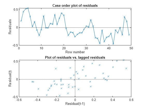
The residuals seem to grow exponentially, and seem autocorrelated (as constructed).

Treat the nonstationary unconditional disturbances by transforming the data appropriately. In this case, take the log of the response series. Difference the logged responses. It is recommended to transform the predictors the same way as the responses to maintain the original interpretation of their relationship. However, do not transform the predictors in this case because they contain negative values. Reestimate the regression model using the transformed responses, and plot the residuals.

dLogY = diff(log(y));
RegMdl2 = fitlm(X(2:end,:),dLogY);

figure
subplot(2,1,1)
plotResiduals(RegMdl2,'caseorder','LineStyle','-')
subplot(2,1,2)
plotResiduals(RegMdl2,'lagged')

h = adftest(RegMdl2.Residuals.Raw)

h = logical
   1

The residual plots indicate that they are still autocorrelated, but stationary. h = 1 indicates that there is enough evidence to suggest that the residual series is not a unit root process.

Once the residuals appear stationary, you can determine the appropriate number of lags for the error model using Box and Jenkins methodology. Then, use regARIMA to completely model the regression model with ARIMA errors.

References

[1] Box, G. E. P., G. M. Jenkins, and G. C. Reinsel. Time Series Analysis: Forecasting and Control. 3rd ed. Englewood Cliffs, NJ: Prentice Hall, 1994.