Simulate States and Observations of Time-Invariant State-Space Model

This example shows how to simulate states and observations of a known, time-invariant state-space model.

Suppose that a latent process is an AR(1) model. The state equation is

where $$u_t$$ is Gaussian with mean 0 and standard deviation 1.

Generate a random series of 100 observations from $$x_t$$, assuming that the series starts at 1.5.

T = 100;
ARMdl = arima('AR',0.5,'Constant',0,'Variance',1);
x0 = 1.5;
rng(1); % For reproducibility
x = simulate(ARMdl,T,'Y0',x0);

Suppose further that the latent process is subject to additive measurement error. The observation equation is

where $${\epsilon }_t$$ is Gaussian with mean 0 and standard deviation 0.75. Together, the latent process and observation equations compose a state-space model.

Use the random latent state process (x) and the observation equation to generate observations.

y = x + 0.75*randn(T,1);

Specify the four coefficient matrices.

A = 0.5;
B = 1;
C = 1;
D = 0.75;

Specify the state-space model using the coefficient matrices.

Mdl = ssm(A,B,C,D)

Mdl = 
State-space model type: ssm

State vector length: 1
Observation vector length: 1
State disturbance vector length: 1
Observation innovation vector length: 1
Sample size supported by model: Unlimited

State variables: x1, x2,...
State disturbances: u1, u2,...
Observation series: y1, y2,...
Observation innovations: e1, e2,...

State equation:
x1(t) = (0.50)x1(t-1) + u1(t)

Observation equation:
y1(t) = x1(t) + (0.75)e1(t)

Initial state distribution:

Initial state means
 x1 
  0 

Initial state covariance matrix
     x1   
 x1  1.33 

State types
     x1     
 Stationary 

Mdl is an ssm model. Verify that the model is correctly specified using the display in the Command Window. The software infers that the state process is stationary. Subsequently, the software sets the initial state mean and covariance to the mean and variance of the stationary distribution of an AR(1) model.

Simulate one path each of states and observations. Specify that the paths span 100 periods.

[simY,simX] = simulate(Mdl,100);

simY is a 100-by-1 vector of simulated responses. simX is a 100-by-1 vector of simulated states.

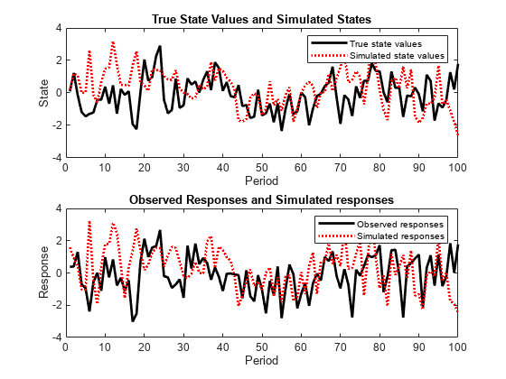
Plot the true state values with the simulated states. Also, plot the observed responses with the simulated responses.

figure
subplot(2,1,1)
plot(1:T,x,'-k',1:T,simX,':r','LineWidth',2)
title({'True State Values and Simulated States'})
xlabel('Period')
ylabel('State')
legend({'True state values','Simulated state values'})
subplot(2,1,2)
plot(1:T,y,'-k',1:T,simY,':r','LineWidth',2)
title({'Observed Responses and Simulated responses'})
xlabel('Period')
ylabel('Response')
legend({'Observed responses','Simulated responses'})

By default, simulate simulates one path for each state and observation in the state-space model. To conduct a Monte Carlo study, specify to simulate a large number of paths.

See Also

ssm | simulate

Related Topics

• Explicitly Create State-Space Model Containing Known Parameter Values
• Simulate Time-Varying State-Space Model