Implement Hardware-Efficient Real Partial-Systolic Matrix Solve Using QR Decomposition with Diagonal Loading
This example shows how to implement a hardware-efficient least-squares solution to the real-valued matrix equation
![$$\left[\begin{array}{c}\lambda I\\A\end{array}\right] X = \left[\begin{array}{c}O\\B\end{array}\right]$$](../../examples/fixedpoint/win64/RealPartialSystolicQRDiagonalLoadingMatrixSolveExample_eq13421924873373409154.png)
using the Real Partial-Systolic Matrix Solve Using QR Decomposition block. This method is known as diagonal loading, and  is known as a regularization parameter.
Diagonal Loading Method
When you set the regularization parameter to a non-zero value in block Real Partial-Systolic Matrix Solve Using QR Decomposition, then the block computes the least-squares solution to
where  is an n-by-n identity matrix and
  is an array of zeros of size n-by-p.
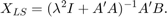
This method is known as diagonal loading, and is known as a regularization parameter. The familiar textbook least-squares solution for this equation is the following, which is derived by multiplying both sides of the equation by ![$[\lambda I,\; A']$](../../examples/fixedpoint/win64/RealPartialSystolicQRDiagonalLoadingMatrixSolveExample_eq17713795801863575823.png) and taking the inverse of the matrix on the left-hand side.
and taking the inverse of the matrix on the left-hand side.
Real Partial-Systolic Matrix Solve Using QR Decomposition block computes the solution efficiently without computing an inverse by computing the QR decomposition, transforming
![$$\left[\begin{array}{c}\lambda I\\A\end{array}\right]$$](../../examples/fixedpoint/win64/RealPartialSystolicQRDiagonalLoadingMatrixSolveExample_eq04204039264175687888.png)
in-place to upper-triangular R, and transforming
![$$\left[\begin{array}{c}O\\B\end{array}\right]$$](../../examples/fixedpoint/win64/RealPartialSystolicQRDiagonalLoadingMatrixSolveExample_eq15030873216691328927.png)
in-place to
![$$C = Q'\left[\begin{array}{c}O\\B\end{array}\right]$$](../../examples/fixedpoint/win64/RealPartialSystolicQRDiagonalLoadingMatrixSolveExample_eq17485136644078923159.png)
and solving the transformed equation  .
.
Define Matrix Dimensions
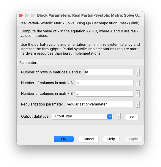
Specify the number of rows in matrices A and B, the number of columns in matrix A, and the number of columns in matrix B.
m = 300; % Number of rows in matrices A and B
n = 10;  % Number of columns in matrix A
p = 1;   % Number of columns in matrix B
Define the Regularization Parameter
When the regularization parameter is non-zero in block Real Partial-Systolic Matrix Solve Using QR Decomposition, then the diagonal-loading method is used. When the regularization parameter is zero, then the equations reduce to the regular least-squares formula AX=B.
regularizationParameter = 1e-3;
Block Parameters
Generate Random Least-Squares Matrices
For this example, use the helper function realRandomLeastSquaresMatrices to generate random matrices A and B for the least-squares problem AX=B. The matrices are generated such that the elements of A and B are between -1 and +1, and A has rank r.
rng('default')
r = 3;   % Rank of matrix A
[A,B] = fixed.example.realRandomLeastSquaresMatrices(m,n,p,r);
Select Fixed-Point Data Types
Use the helper function realQRMatrixSolveFixedpointTypes to select fixed-point data types for input matrices A and B, and output X such that there is a low probability of overflow during the computation.
max_abs_A = 1;       % Upper bound on max(abs(A(:))
max_abs_B = 1;       % Upper bound on max(abs(B(:))
precisionBits = 24;  % Number of bits of precision
T = fixed.realQRMatrixSolveFixedpointTypes(m,n,max_abs_A,max_abs_B,precisionBits);
A = cast(A,'like',T.A);
B = cast(B,'like',T.B);
OutputType = fixed.extractNumericType(T.X);
Open the Model
model = 'RealPartialSystolicQRDiagonalLoadingMatrixSolveModel';
open_system(model);

The Data Handler subsystem in this model takes real matrices A and B as inputs. The ready port triggers the Data Handler. After sending a true validIn signal, there may be some delay before ready is set to false. When the Data Handler detects the leading edge of the ready signal, the block sets validIn to true and sends the next row of A and B. This protocol allows data to be sent whenever a leading edge of the ready signal is detected, ensuring that all data is processed.
Set Variables in the Model Workspace
Use the helper function setModelWorkspace to add the variables defined above to the model workspace. These variables correspond to the block parameters for the Real Partial-Systolic Matrix Solve Using QR Decomposition block.
numSamples = 1; % Number of sample matrices
fixed.example.setModelWorkspace(model,'A',A,'B',B,'m',m,'n',n,'p',p,...
    'regularizationParameter',regularizationParameter,...
    'numSamples',numSamples,'OutputType',OutputType);
Simulate the Model
out = sim(model);
Construct the Solution from the Output Data
The Real Partial-Systolic Matrix Solve Using QR Decomposition block outputs data one row at a time. When a result row is output, the block sets validOut to true. The rows of X are output in the order they are computed, last row first, so you must reconstruct the data to interpret the results. To reconstruct the matrix X from the output data, use the helper function matrixSolveModelOutputToArray.
X = fixed.example.matrixSolveModelOutputToArray(out.X,n,p,numSamples);
Verify the Accuracy of the Output
To evaluate the accuracy of the Real Partial-Systolic Matrix Solve Using QR Decomposition block, compute the relative error.
A_lambda = [regularizationParameter * eye(n);A];
B_0 = [zeros(n,p);B];
relative_error = norm(double(A_lambda*X - B_0))/norm(double(B_0)) %#ok<NOPTS>
relative_error =

   1.2199e-04
See Also
Tools
Blocks
Topics
- Implement Hardware-Efficient Real Partial-Systolic Matrix Solve Using QR Decomposition
- Implement Hardware-Efficient Real Partial-Systolic Matrix Solve Using QR Decomposition with Tikhonov Regularization
- Algorithms to Determine Fixed-Point Types for Real Least-Squares Matrix Solve AX=B
- Determine Fixed-Point Types for Real Least-Squares Matrix Solve AX=B
- Determine Fixed-Point Types for Real Least-Squares Matrix Solve with Tikhonov Regularization