Design Controller for Artificial Pancreas Using Fuzzy Logic

Video Walkthrough

For a walkthough of the example, watch the video.

Background

Type 1 diabetes is a widespread health problem that occurs when the pancreas fails to produce enough insulin to regulate blood glucose levels. An uncontrolled high blood glucose level (hyperglycemia) can cause significant damage to the human body. Therefore, an artificial pancreas system that continuously monitors and regulates blood glucose level with appropriate subcutaneous insulin infusion is a major goal in healthcare device development.

The following figure, which is adapted from [1], shows the components of an artificial pancreas system.

The continuous glucose monitoring system periodically measures the blood glucose level of the diabetic patient and passes this information to a controller. The controller drives an insulin pump, which injects an optimal insulin dosage to the patient, thus regulating the blood glucose level. The controller provides the following two types of insulin dosage.

Therefore, the task for the controller is to generate corrective insulin doses for the following cases.

Artificial Pancreas Model

The artificialPancreasWithFISTreeControl Simulink® model implements an artificial pancreas system.

model = "artificialPancreasWithFISTreeControl";
load_system(model)

This model contains the following subsystems.

To view how the blood glucose level of a diabetic patient changes when the body absorbs glucose without corrective insulin infusion, simulate the model with a constant zero control action. To do so, open the control loop by setting closeLoop to 0.

closeLoop = 0;
openLoopOutput = sim(model);
plotAbsorbedAndBloodGlucose(openLoopOutput)

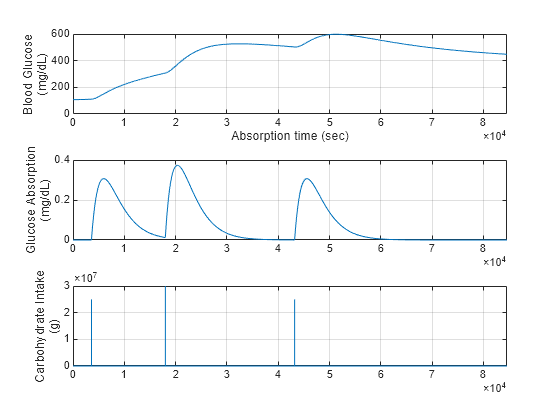
Without corrective insulin infusion, the patient blood glucose level increases and remains in a hyperglycemic state.

Close the control loop for tuning and simulation.

closeLoop = 1;

Create FIS Tree Controller Structure

The controller has the following inputs, as described in [4].

The output of the controller is an optimal insulin infusion dosage that maintains the blood glucose level of a diabetic patient at a normal level.

To produce an optimal insulin dosage based on the observed inputs, the fuzzy controller described in [4] uses expert knowledge to construct a single FIS with 75 rules. However, creating a large rule base using expert knowledge is a complicated process due to the manual construction of each fuzzy rule for all combinations of input membership functions (MFs).

Alternatively, using a FIS tree produces a system with multiple FISs, each with a smaller rule base. The hierarchical structure of the FIS tree and the smaller rule bases allow for a more intuitive understanding of the inference process.

This example uses an incremental design approach to combine the controller inputs using two Mamdani FIS objects in an incremental tree structure. For more information on fuzzy tree structures, see FIS Trees.

The blood glucose level and its rate of change both contribute more to the control actions compared to the acceleration rate, which is often small and can create noise in the output. Therefore, in the first level of the FIS tree, you precalculate the insulin infusion rate Precalculated_Dose by combining the effects of the blood glucose level BG_Level and its rate of change BG_Rate. The acceleration rate BG_Accel is included in the second layer of the FIS tree.

Create the FIS (fis1) for the first level of the tree structure. The inputs of fis1 each use three uniformly distributed triangular MFs. The output of fis1 uses five such MFs, named as follows:

Specify the maximum dose level.

maxDose = 2;

Define membership function names for the input variables.

mfNames1 = ["L","M","H"]; % Low, Medium, High
mfNames2 = ["N","Z","P"]; % Negative, Zero, Positive

Create first FIS.

fis1 = mamfis(Name="fis1",NumInputs=2,NumOutputs=1, ...
    NumInputMFs=3,NumOutputMFs=5);

Configure the input and output variables of the FIS using the updateFISInput and updateFISOutput helper functions included at the end of this example.

fis1 = updateFISInput(fis1,1,"BG_Level",[80 120],mfNames1);
fis1 = updateFISInput(fis1,2,"BG_Rate",[-0.5 0.5],mfNames2);
fis1 = updateFISOutput(fis1,1,"Precalculated_Dose",[0 maxDose]);

Plot the FIS.

figure
plotfis(fis1)

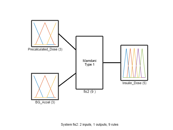
Create the FIS (fis2) for the second level of the tree. Using fis2, you generate the final insulin dosage by combining the precalculated dose from the first layer with the effect of the blood glucose acceleration rate. In this case, the inputs and the output also use three and five uniformly distributed triangular MFs, respectively.

fis2 = mamfis(Name="fis2",NumInputs=2,NumOutputs=1, ...
    NumInputMFs=3,NumOutputMFs=5);

Configure the input and output variables of the second FIS.

fis2 = updateFISInput(fis2,1,"Precalculated_Dose",[0 maxDose],mfNames1);
fis2 = updateFISInput(fis2,2,"BG_Accel",[-0.005 0.005],mfNames2);
fis2 = updateFISOutput(fis2,1,"Insulin_Dose",[0 maxDose]);

Plot the second FIS.

figure
plotfis(fis2)

Combine fis1 and fis2 into a FIS tree structure.

connection = [fis1.Name + "/" + fis1.Outputs(1).Name ...
    fis2.Name + "/" + fis2.Inputs(1).Name];
fisTInit = fistree([fis1 fis2],connection);

figure
plotfis(fisTInit)

The initial fuzzy systems are constructed with default fuzzy rules that are not tuned to produce optimal insulin dosages.

Tune Controller Rules

Once you have a FIS tree structure, you can optimize the controller behavior by tuning the rules and MF parameters of the component FIS objects. To do so, you can use the tunefis function.

In general, uniformly distributed MFs provide a meaningful initial condition for tuning a fuzzy system. Therefore, as an initial tuning step, you can learn the rules of the FIS objects while keeping their default MF parameters.

To learn the rules, first get the tunable settings from the fuzzy systems.

[in,out,rule] = getTunableSettings(fisTInit);

Next, update the rule settings to optimize only the rule consequents. By doing so, you keep the existing rule antecedents, which already include all possible input MF combinations for their corresponding FIS inputs.

for rId = 1:numel(rule)
    rule(rId).Antecedent.Free = false;    
end

Create an option set for the tuning process.

options = tunefisOptions;

Use the default genetic algorithm tuning method for learning the rules. Set the maximum number of generations to 3 and use a population size of 100.

options.MethodOptions.MaxGenerations = 3;
options.MethodOptions.PopulationSize = 100;

Next, create a cost function to evaluate each candidate rule base. At the end of the optimization process, the rule base with the minimum cost is selected for the fuzzy systems in the FIS tree.

For this example, the cost function (costFcn.m) simulates the artificialPancreasWithFISTreeControl model using the candidate rule base. Using the resulting simulation output, the cost function computes the cost using the following steps.

Using this cost function, the tuning process selects rule bases that maintain a normal condition and avoid high glucose levels. Also, the high error values used in step 2 help discard rule bases that produce low blood glucose levels.

% Specify the nominal and minimum glucose levels.
refLevel = 90;
minLevel = 80;

% Calculate error from the nominal value.
err = glucose - refLevel;

% Specify high error values for the glucose levels below the nominal level.
err(glucose<minLevel) = 100;

% Calculate cost as the root mean square of the error.
errSquare = err.^2;
meanSquare = mean(errSquare);
cost = sqrt(meanSquare);

Tuning is a time-consuming process, so for this example, load a pretuned FIS tree. To tune the FIS tree yourself instead, set runtunefis to true.

runtunefis = false;

Load pretuned FIS tree data.

data = load("fuzzyPancreasExampleData.mat");

minData = MinCostData;
wsVars = ["fisT" "closeLoop"];
minLevel = 80;
refLevel = 90;
if runtunefis
    rng("default")
    fisTRuleTuned = tunefis(fisTInit,rule,...
        @(fis)costFcn(fis,model,minLevel,refLevel,wsVars,minData),options);
else
    fisTRuleTuned = data.fisTRuleTuned;
    minCost = costFcn(fisTRuleTuned,model,minLevel,refLevel,wsVars)
end

minCost = 
26.3335

Simulate the model using the FIS tree with tuned rule bases.

fisT = fisTRuleTuned;
ruleTunedOutput = sim(model);

Plot the resulting regulated glucose levels and insulin infusion rate.

plotGlucoseAndInsulin(ruleTunedOutput,...
    "Blood Glucose and Insulin Dosage with Learned Rule Base")

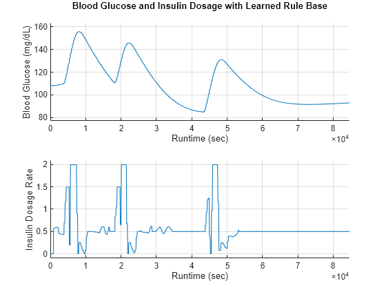
With the tuned rule base, the glucose level is now maintained below 160 mg/dL, and it settles close to 90 mg/dL after the third meal. The controller generates a short-term high insulin dosage (bolus mode) at each meal time and a long-term reduced insulin dosage (basal mode) during the fasting periods.

Analyze and Modify Rule Base

To visualize the behavior of the tuned rule base, plot the control surface of each fuzzy system in the FIS tree.

figure(Position=[300 300 600 300]);
subplot(1,2,1)
gensurf(fisTRuleTuned.FIS(1))
title("Control Surface - fis1")
subplot(1,2,2)
gensurf(fisTRuleTuned.FIS(2))
title("Control Surface - fis2")

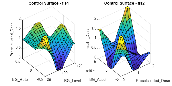
The following tables show the corresponding rule bases of fis1 and fis2.

showRuleBase(fisTRuleTuned.FIS(1))

Rule base of fis1:
                         BG_Rate: N               BG_Rate: Z                BG_Rate: P      
                   ______________________    _____________________    ______________________

    BG_Level: L    Precalculated_Dose: VH    Precalculated_Dose: M    Precalculated_Dose: M 
    BG_Level: M    Precalculated_Dose: VL    Precalculated_Dose: M    Precalculated_Dose: H 
    BG_Level: H    Precalculated_Dose: M     Precalculated_Dose: H    Precalculated_Dose: VL

showRuleBase(fisTRuleTuned.FIS(2))

Rule base of fis2:
                               BG_Accel: N         BG_Accel: Z         BG_Accel: P   
                             ________________    ________________    ________________

    Precalculated_Dose: L    Insulin_Dose: VH    Insulin_Dose: VL    Insulin_Dose: H 
    Precalculated_Dose: M    Insulin_Dose: VL    Insulin_Dose: L     Insulin_Dose: L 
    Precalculated_Dose: H    Insulin_Dose: L     Insulin_Dose: VL    Insulin_Dose: VH

These tables show that some of the control actions are nonintuitive. For example:

Update the rules by modifying their consequent values.

% Update fis1 rules.
fisTRuleUpdate = fisTRuleTuned;
fisTRuleUpdate.FIS(1).Rules(1).Description = ...
    "BG_Level==L & BG_Rate==N => Precalculated_Dose=VL";
fisTRuleUpdate.FIS(1).Rules(2).Description = ...
    "BG_Level==M & BG_Rate==N => Precalculated_Dose=M";
fisTRuleUpdate.FIS(1).Rules(3).Description = ...
    "BG_Level==H & BG_Rate==N => Precalculated_Dose=H";
fisTRuleUpdate.FIS(1).Rules(9).Description = ...
    "BG_Level==H & BG_Rate==P => Precalculated_Dose=VH";

% Update fis2 rules.
fisTRuleUpdate.FIS(2).Rules(1).Description = ...
    "Precalculated_Dose==L & BG_Accel==N => Insulin_Dose=VL";
fisTRuleUpdate.FIS(2).Rules(3).Description = ...
    "Precalculated_Dose==H & BG_Accel==N => Insulin_Dose=M";
fisTRuleUpdate.FIS(2).Rules(6).Description = ...
    "Precalculated_Dose==H & BG_Accel==Z => Insulin_Dose=M";
fisTRuleUpdate.FIS(2).Rules(7).Description = ...
    "Precalculated_Dose==L & BG_Accel==P => Insulin_Dose=L";

View the modified rule bases.

showRuleBase(fisTRuleUpdate.FIS(1))

Rule base of fis1:
                         BG_Rate: N               BG_Rate: Z                BG_Rate: P      
                   ______________________    _____________________    ______________________

    BG_Level: L    Precalculated_Dose: VL    Precalculated_Dose: M    Precalculated_Dose: M 
    BG_Level: M    Precalculated_Dose: M     Precalculated_Dose: M    Precalculated_Dose: H 
    BG_Level: H    Precalculated_Dose: H     Precalculated_Dose: H    Precalculated_Dose: VH

showRuleBase(fisTRuleUpdate.FIS(2))

Rule base of fis2:
                               BG_Accel: N         BG_Accel: Z         BG_Accel: P   
                             ________________    ________________    ________________

    Precalculated_Dose: L    Insulin_Dose: VL    Insulin_Dose: VL    Insulin_Dose: L 
    Precalculated_Dose: M    Insulin_Dose: VL    Insulin_Dose: L     Insulin_Dose: L 
    Precalculated_Dose: H    Insulin_Dose: M     Insulin_Dose: M     Insulin_Dose: VH

Visualize the resulting FIS control surfaces.

figure(Position=[300 300 600 300]);
subplot(1,2,1)
gensurf(fisTRuleUpdate.FIS(1))
title("Control Surface - fis1")
subplot(1,2,2)
gensurf(fisTRuleUpdate.FIS(2))
title("Control Surface - fis2")

The control surfaces correspond to a more intuitive controller behavior.

To check if the updated rules improve the controller performance, simulate the model and plot the results. Compare the results with those of the controller with tuned MF parameters.

fisT = fisTRuleUpdate;
ruleUpdatedOutput = sim(model);

plotGlucoseAndInsulin([ruleTunedOutput ruleUpdatedOutput],...
    "Blood Glucose and Insulin Dosage with Updated Rule Base",...
    ["Learned rules","Updated rules"])

The controller with updated rules reduces the blood glucose levels compared to the tuned FIS tree controller.

Updating the rules reduces the value of the cost function.

minCost = costFcn(fisTRuleUpdate,model,minLevel,refLevel,wsVars)

minCost = 
23.2702

Tune Membership Function Parameters

To further improve the controller performance, you can tune the MF parameters of the FIS tree.

To do so, use a local optimization method, such as pattern search. For this example, set the maximum number of optimization iterations to 10.

options.Method = "patternsearch";
options.MethodOptions.MaxIterations = 10;

By default, each input variable has three uniformly distributed triangular MFs. For example, view the MFs for the first input of fis1.

figure
plotmf(fisTRuleUpdate.FIS(1),"input",1)

Configure the tunable settings for the input variables such that the leftmost and rightmost peaks remain unchanged during tuning.

for i = 1:4
    in(i).MembershipFunctions(1).Parameters.Free = [0 0 1];
    in(i).MembershipFunctions(end).Parameters.Free = [1 0 0];
end

Similarly, configure the tunable settings for the output variables. Each output variable has five triangular membership functions.

for i = 1:2
    out(i).MembershipFunctions(1).Parameters.Free = [0 0 1];
    out(i).MembershipFunctions(end).Parameters.Free = [1 0 0];
end

Tune the MF parameter values using the updated tunable settings.

if runtunefis
    figure
    reset(minData)
    rng("default")
    fisTMFTuned = tunefis(fisTRuleUpdate,[in;out],...
        @(fis)costFcn(fis,model,minLevel,refLevel,wsVars,minData),options);
else
    fisTMFTuned = data.fisTMFTuned;
    minCost = costFcn(fisTMFTuned,model,minLevel,refLevel,wsVars)
end

minCost = 
20.9651

The MF tuning process reduces the value of the cost function further.

Simulate the model using the controller with tuned MF parameters.

fisT = fisTMFTuned;
mfTunedOutput = sim(model);

Plot the resulting regulated glucose levels and insulin infusion rate. Compare the results with those for the controller with tuned rule bases.

plotGlucoseAndInsulin([ruleUpdatedOutput mfTunedOutput],...
    "Blood Glucose and Insulin Dosage with Tuned MFs",...
    ["Updated rules","Tuned MFs"])

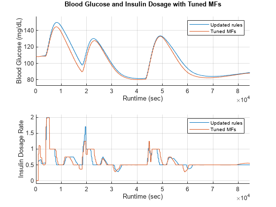
The tuned MF parameters improve the performance and reduce the minimum cost value.

To further improve controller performance you can implement the following modifications.

References

[1] Grant, Paul. “A New Approach to Diabetic Control: Fuzzy Logic and Insulin Pump Technology.” Medical Engineering & Physics 29, no. 7 (September 2007): 824–27. https://doi.org/10.1016/j.medengphy.2006.08.014.

[2] Wilinska, M.E., L.J. Chassin, H.C. Schaller, L. Schaupp, T.R. Pieber, and R. Hovorka. “Insulin Kinetics in Type-1 Diabetes: Continuous and Bolus Delivery of Rapid Acting Insulin.” IEEE Transactions on Biomedical Engineering 52, no. 1 (January 2005): 3–12. https://doi.org/10.1109/TBME.2004.839639.

[3] Hovorka, Roman, Valentina Canonico, Ludovic J Chassin, Ulrich Haueter, Massimo Massi-Benedetti, Marco Orsini Federici, Thomas R Pieber, et al. “Nonlinear Model Predictive Control of Glucose Concentration in Subjects with Type 1 Diabetes.” Physiological Measurement 25, no. 4 (August 1, 2004): 905–20. https://doi.org/10.1088/0967-3334/25/4/010.

[4] Mauseth, Richard, Youqing Wang, Eyal Dassau, Robert Kircher, Donald Matheson, Howard Zisser, Lois Jovanovič, and Francis J. Doyle. “Proposed Clinical Application for Tuning Fuzzy Logic Controller of Artificial Pancreas Utilizing a Personalization Factor.” Journal of Diabetes Science and Technology 4, no. 4 (July 2010): 913–22. https://doi.org/10.1177/193229681000400422.

Helper Functions

function fis = updateFISInput(fis,id,name,range,mfNames)
% Update FIS input with the specified parameter values.

fis.Inputs(id).Name = name;
fis.Inputs(id).Range = range;

for mfId = 1:length(mfNames)
    fis.Inputs(id).MembershipFunctions(mfId).Name = mfNames(mfId);
    params = range(1) + ...
        diff(range)*fis.Inputs(id).MembershipFunctions(mfId).Parameters;
    fis.Inputs(id).MembershipFunctions(mfId).Parameters = params;
end

end

function fis = updateFISOutput(fis,id,name,range)
% Update FIS output with the specified parameter values.

rangeDiff = diff(range);
fis.Outputs(id).Name = name;

% MF names - Very Low, Low, Medium, High, Very High
mfNames = [...
    "VL","L","M","H","VH"];

for mfId = 1:length(mfNames)
    fis.Outputs(id).MembershipFunctions(mfId).Name = mfNames(mfId);
    params = range(1) + ...
        rangeDiff*fis.Outputs(id).MembershipFunctions(mfId).Parameters;
    fis.Outputs(id).MembershipFunctions(mfId).Parameters = params;
end

% Extend output range values to fit the output MFs.
left = fis.Outputs(id).MembershipFunctions(1).Parameters(1);
right = fis.Outputs(id).MembershipFunctions(end).Parameters(end);
fis.Outputs(id).Range = [left right];

end