Explainable Fuzzy Support System for Black-Box Model of Robot Obstacle Avoidance

This example uses:

This example shows how to develop a support fuzzy inference system to explain the behavior of a black-box model when the original data used to train the black-box model is not available.

Using nondeterministic machine learning methods, such as reinforcement learning, you can design a black-box model to estimate the input-output mapping for a given set of experimental or simulation data. However, the input-output relationship defined by such a black-box model is difficult to understand.

In general, users are unable to explain the causal relations from the inputs to the outputs. Also, they are unable to change the system behavior using the implicit input-output models. To resolve these problems, a common approach is to create a transparent support system for the black-box model. The goal of such a support system is to help users understand and explain the input-output relationships developed in a black box model.

A fuzzy inference system (FIS) is a transparent model that represents system knowledge using an explainable rule base. Since the rule base of a fuzzy system is easier for a user to intuitively understand, a FIS is often used as a support system to explain an existing black-box model.

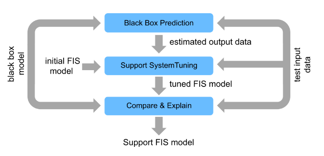
The following figure shows the general steps for developing a fuzzy support system from an existing black-box model when the original training data for the black-box model is not available.

Generate black-box model outputs for a given set of test data.
Tune a FIS using the test input data and generated output data.
Finally, compare the performance of the models and explain the black-box predictions using the FIS.

In general, you can use a fuzzy support system to explain different types of black-box models. For this example, the black-box model is implemented using a reinforcement learning (RL) agent, which requires Reinforcement Learning Toolbox™ software.

Navigation Environment

The RL agent in this example is trained to navigate a robot in a simulation environment while avoiding obstacles. The navigation environment is described in Tune Fuzzy Robot Obstacle Avoidance System Using Custom Cost Function.

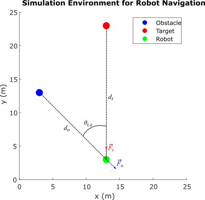
The environment describes a navigation task to reach a specified target while avoiding obstacles. The direction to the target is represented as a unit force vector ( $\vec{F_{t}}$ ) directed from the robot to a target location. The obstacle avoidance direction is represented by a unit force vector ( $\vec{F_{o}}$ ) directed towards the robot from the closest obstacle location. The robot, target, and obstacle are shown as circles with 0.5 m radius in the 25 m x 25 m simulation environment. The navigation task is to combine the force vectors such that the direction $θ$ of the resultant force vector $\vec{F}$ provides a collision-free direction for the robot.

$\vec{F} = w \vec{F_{o}} + (1 - w) \vec{F_{t}}$ , where $0 \leq w \leq 1$

$θ = ∠ \vec{F}$

The weight $w$ of the force vector $\vec{F_{o}}$ is calculated using function $f_{w}$ .

$w = f_{w} (α, θ_{t, o})$

Here:

$α = \frac{d_{o}}{d_{t}}$ is the ratio of the robot-to-obstacle distance ( $d_{o}$ ) and the robot-to-target-distance ( $d_{t}$ )
$θ_{t, o}$ is the absolute difference between the target and obstacle directions with respect to the robot

The RL agent learns a policy to model $f_{w}$ for collision-free robot navigation in the environment using $(α, θ_{t, o})$ as the observation and $w$ as the action.

Policy Simulation

To simulate the learned policy, first load the trained RL agent.

rlmodel = load("rlNavModel.mat");
trainedAgent = rlmodel.trainedAgent;

Create the simulation environment using an RL environment object as defined in the NavigationEnvironment.m helper file. This environment definition also includes several helper functions used in this example.

env = NavigationEnvironment;

Simulate the agent in the navigation environment.

sim(trainedAgent,env)

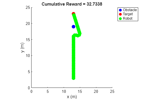
Figure Mobile robot navigation with collision avoidance contains an axes object. The axes object with title Cumulative Reward = 32.7338, xlabel x (m), ylabel y (m) contains 135 objects of type line, rectangle. One or more of the lines displays its values using only markers These objects represent Obstacle, Target, Robot.

The trained RL agent successfully avoids obstacles using a learned policy.

However, the agent does not provide an explanation about how it avoids the obstacle. The actor of the agent uses a deep neural network (DNN) model, which encapsulates the navigation policy in terms of hidden units and their associated parameters. As an example, you can directly simulate the actor of the agent to generate an action for a specific observation as follows.

alpha = 0.1;
theta = 0;
obstacleWeight = trainedAgent.getAction([alpha;theta])

obstacleWeight = 1x1 cell array
    {[0.9253]}

The actor produces a high weight for obstacle avoidance. However, it does not provide any tools to explain how the knowledge is represented in the model and how it has been used to generate the action in this case.

Generate Test Data

To explain the agent actions, you can develop a fuzzy support system using a data-driven approach. To do so, you must first generate input-output training data using different test cases, where each case represents different direction of the robot. For $n$ test cases, the robot direction is specified as $\pm \frac{2 π}{n}$ rad. In each case, the target, obstacle, and the robot are located along the same line. However, their relative distances are varied randomly.

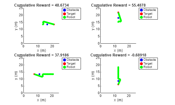
Generate four test cases using the createTestCases helper function. You can visualize the test cases using the showTestCases helper function.

numTestCases = 4;
rng("default")
testCases = createTestCases(env,numTestCases);
showTestCases(env,testCases)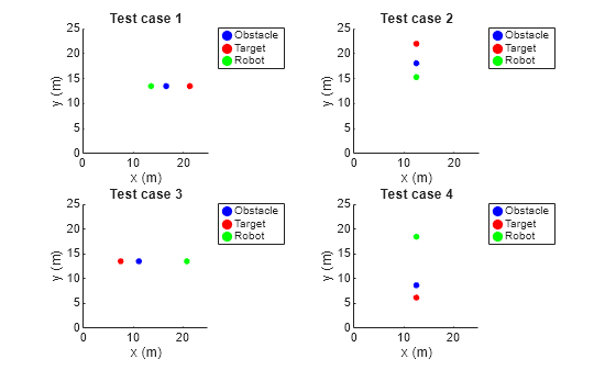

Use the test cases to generate input-output training data for the fuzzy system using the generateData helper function.

[X,Y] = generateData(env,trainedAgent,testCases);

Create and Tune Support System

To define the fuzzy support system, you must create and tune a FIS.

Create Initial FIS

Create a Mamdani fuzzy inference system.

fisin = mamfis;

Add two input variables for the observations. Each input includes two linear saturation membership functions (MFs).

numMFs = 2;
% Input 1
fisin = addInput(fisin,[0 2],"Name","alpha","NumMFs",numMFs);
fisin.Inputs(1).MembershipFunctions(1).Type = "linzmf";
fisin.Inputs(1).MembershipFunctions(end).Type = "linsmf";

% Input 2
fisin = addInput(fisin,[0 pi/2],"Name","theta_t_o","NumMFs",numMFs);
fisin.Inputs(2).MembershipFunctions(1).Type = "linzmf";
fisin.Inputs(2).MembershipFunctions(end).Type = "linsmf";

Add an output variable for the action, which represents the weight (priority) of obstacle avoidance. Add output MFs for all possible combinations of input MFs.

numOutMFs = numMFs^2;
fisin = addOutput(fisin,[0 1],"Name","w","NumMFs",numOutMFs);

Next, add default rules for all combinations of input MFs. The default rules always produce a low weight for obstacle avoidance.

[in1,in2] = ndgrid(1:numMFs,1:numMFs);
rules = [in1(:) in2(:) ones(numOutMFs,3)];
fisin = addRule(fisin,rules);

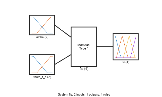
Show the initial FIS.

figure
plotfis(fisin)

Tune FIS

To train the FIS, use the following two stages.

Learn the rule base to establish the input-output relationships.
Tune the membership function parameters for the input and output variables.

To tune the rules, first obtain the rule parameter settings from the FIS.

[~,~,rule] = getTunableSettings(fisin);

Since you have a rule for each possible input combination, configure the training settings to keep the rule antecedents fixed. As a result, tuning will only modify the rule consequents.

for ct = 1:length(rule)
    rule(ct).Antecedent.Free = 0;
end

Create an option set for tuning and specify particleswarm as the tuning method. Set maximum number of tuning iterations to 50.

options = tunefisOptions("Method","particleswarm");
options.MethodOptions.MaxIterations = 50;

Tuning is a time-consuming process. For this example, load a pretrained FIS by setting runtunefis to false. To tune the FIS yourself instead, set runtunefis to true.

runtunefis = false;

Tune the fuzzy rules. For reproducibility, reset the random number generator using the default seed.

if runtunefis
    rng("default")
    fisR = tunefis(fisin,rule,X,Y,options);
else
    data = load("flNavModel.mat");
    fisR = data.fisR;
end

Display the tuned rules.

disp([fisR.Rules.Description]')

    "alpha==mf1 & theta_t_o==mf1 => w=mf2 (1)"
    "alpha==mf2 & theta_t_o==mf1 => w=mf1 (1)"
    "alpha==mf1 & theta_t_o==mf2 => w=mf1 (1)"
    "alpha==mf2 & theta_t_o==mf2 => w=mf1 (1)"

Output membership functions 3 and 4 are not used in the rule base. Remove these membership functions from the output variable.

fisR.Outputs(1).MembershipFunctions(3:4) = [];

Next, tune the input and output MF parameters. To do so, first obtain the corresponding tunable settings from the FIS.

[in,out] = getTunableSettings(fisR);

For this tuning step, use the patternsearch algorithm fine tuning of the MF parameters and set maximum number of iterations number to 100.

options.Method = "patternsearch";
options.MethodOptions.MaxIterations = 100;

Tune the MF parameters.

if runtunefis
    rng("default")
    fisMF = tunefis(fisR,[in;out],X,Y,options);
else
    fisMF = data.fisMF;
end

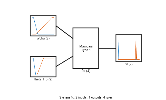
Show the tuned fuzzy system.

fisout = fisMF;
figure
plotfis(fisout)

Simulate Fuzzy System

Validate the tuned FIS for the test cases using the simTestCasesWithFIS helper function.

simTestCasesWithFIS(env,fisout,testCases)

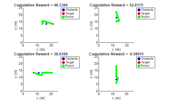
The tuned fuzzy system generates similar reward values for the test cases as compared to the RL agent.

Explain Black-Box Model

With a trained support system, you can now explain the behavior of the black-box model.

Explainable Rule Base with Meaningful MF Names

For interpretability, first, specify names of the MFs for each input and output variable as low and high.

fisout.Inputs(1).MembershipFunctions(1).Name = "low";
fisout.Inputs(1).MembershipFunctions(2).Name = "high";
fisout.Inputs(2).MembershipFunctions(1).Name = "low";
fisout.Inputs(2).MembershipFunctions(2).Name = "high";
fisout.Outputs(1).MembershipFunctions(1).Name = "low";
fisout.Outputs(1).MembershipFunctions(2).Name = "high";

View the tuned rules with the updated names.

disp([fisout.Rules.Description]')

    "alpha==low & theta_t_o==low => w=high (1)"
    "alpha==high & theta_t_o==low => w=low (1)"
    "alpha==low & theta_t_o==high => w=low (1)"
    "alpha==high & theta_t_o==high => w=low (1)"

Using these rules, you can explain the behavior of the RL agent.

In the first rule, when $α$ is low (the obstacle is located closer to the robot as compared to the target) and $θ_{t, o}$ is low (the obstacle and target are located in the same direction), the robot should actively avoid the obstacle. In this case, collision avoidance has a higher priority than reaching the target.
In the second rule, when $α$ is high (both the obstacle and the target are located away from the robot) and $θ_{t, o}$ is low (the obstacle and target are located in the same direction), the robot can still move towards the target to optimize the travel distance. In this case, reaching the target has a higher priority than collision avoidance.
In the third and fourth rules, $θ_{t, o}$ is high (the obstacle and target are located in different directions). In this case, the robot can always safely navigate towards the target. Therefore, reaching the target has a higher priority than collision avoidance.

Overall, the black-box action (collision avoidance weight) is explainable using the rule base of the fuzzy support system.

Visualization of Observation-to-Action Mapping

The control surface of the fuzzy system describes observations (input) to actions (output) mapping according to the rule base.

figure
gensurf(fisMF)

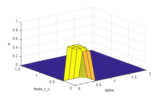
Figure contains an axes object. The axes object with xlabel alpha, ylabel theta indexOf to baseline theta_t_o contains an object of type surface.

The fuzzy rule base provides a linguistic relation between the observations and actions; whereas the control surface augments this linguistic relation by adding numeric details for observation-to-action mapping.

Explanation of Runtime Action Selection

You can also use the support system to explain each black-box action generated in a control cycle. The following diagram explains the parallel execution settings of both the black-box model and the support system for run-time explanation of an action.

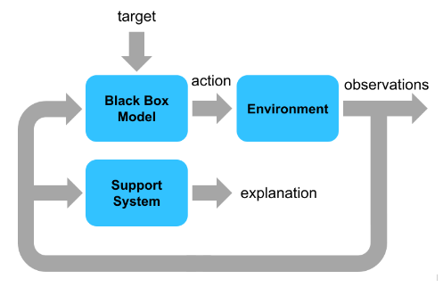
The black-box model and the support system run in parallel and use the same environment observations. The black-box model drives environment changes. The support system observes the environment and explains the black-box action. For this example, the support system explanation includes the following information.

Index of the control cycle
Current observation
Action (obstacle weight) generated by the black-box model and the fuzzy support system
Fuzzy rule that is most is most suitable based on the current observation

The output data format for each control interval is as follows.

========== Control cycle: 1 ========== 
Observations = [0.466667 0], agent output (weight) = 0.582038, FIS output (weight) = 0.545197
Max strength rule: alpha==low & theta_t_o==low => w=high (1)

Simulate the agent and FIS using the compareAgentWithFIS helper function. The results show explanations for each action and the overall navigation trajectory using the black-box model.

setDefaultPositions(env);
[agentActions,fisActions] = compareAgentWithFIS(env,trainedAgent,fisout);

========== Control cycle: 1 ==========
Observations = [0.8 0], agent output (weight) = 0.000371873, FIS output (weight) = 0.0097047
Max strength rule: alpha==high & theta_t_o==low => w=low (1)
========== Control cycle: 2 ==========
Observations = [0.794872 0], agent output (weight) = 0.000371873, FIS output (weight) = 0.00974128
Max strength rule: alpha==high & theta_t_o==low => w=low (1)
========== Control cycle: 3 ==========
Observations = [0.789474 0], agent output (weight) = 0.000409484, FIS output (weight) = 0.0097804
Max strength rule: alpha==high & theta_t_o==low => w=low (1)
========== Control cycle: 4 ==========
Observations = [0.783784 0], agent output (weight) = 0.000453234, FIS output (weight) = 0.00982234
Max strength rule: alpha==high & theta_t_o==low => w=low (1)
========== Control cycle: 5 ==========
Observations = [0.777778 0], agent output (weight) = 0.000504375, FIS output (weight) = 0.00986741
Max strength rule: alpha==high & theta_t_o==low => w=low (1)
========== Control cycle: 6 ==========
Observations = [0.771429 0], agent output (weight) = 0.000564635, FIS output (weight) = 0.00991599
Max strength rule: alpha==high & theta_t_o==low => w=low (1)
========== Control cycle: 7 ==========
Observations = [0.764706 0], agent output (weight) = 0.00063616, FIS output (weight) = 0.0099685
Max strength rule: alpha==high & theta_t_o==low => w=low (1)
========== Control cycle: 8 ==========
Observations = [0.757576 0], agent output (weight) = 0.000721812, FIS output (weight) = 0.01
Max strength rule: alpha==high & theta_t_o==low => w=low (1)
========== Control cycle: 9 ==========
Observations = [0.75 0], agent output (weight) = 0.000842512, FIS output (weight) = 0.01
Max strength rule: alpha==high & theta_t_o==low => w=low (1)
========== Control cycle: 10 ==========
Observations = [0.741935 0], agent output (weight) = 0.000993103, FIS output (weight) = 0.01
Max strength rule: alpha==high & theta_t_o==low => w=low (1)
========== Control cycle: 11 ==========
Observations = [0.733333 0], agent output (weight) = 0.00118306, FIS output (weight) = 0.01
Max strength rule: alpha==high & theta_t_o==low => w=low (1)
========== Control cycle: 12 ==========
Observations = [0.724138 0], agent output (weight) = 0.00142586, FIS output (weight) = 0.01
Max strength rule: alpha==high & theta_t_o==low => w=low (1)
========== Control cycle: 13 ==========
Observations = [0.714286 0], agent output (weight) = 0.00174063, FIS output (weight) = 0.01
Max strength rule: alpha==high & theta_t_o==low => w=low (1)
========== Control cycle: 14 ==========
Observations = [0.703704 0], agent output (weight) = 0.00215521, FIS output (weight) = 0.01
Max strength rule: alpha==high & theta_t_o==low => w=low (1)
========== Control cycle: 15 ==========
Observations = [0.692308 0], agent output (weight) = 0.00271079, FIS output (weight) = 0.01
Max strength rule: alpha==high & theta_t_o==low => w=low (1)
========== Control cycle: 16 ==========
Observations = [0.68 0], agent output (weight) = 0.00346974, FIS output (weight) = 0.01
Max strength rule: alpha==high & theta_t_o==low => w=low (1)
========== Control cycle: 17 ==========
Observations = [0.666667 0], agent output (weight) = 0.00452864, FIS output (weight) = 0.01
Max strength rule: alpha==high & theta_t_o==low => w=low (1)
========== Control cycle: 18 ==========
Observations = [0.652174 0], agent output (weight) = 0.00657335, FIS output (weight) = 0.01
Max strength rule: alpha==high & theta_t_o==low => w=low (1)
========== Control cycle: 19 ==========
Observations = [0.636364 0], agent output (weight) = 0.00989613, FIS output (weight) = 0.01
Max strength rule: alpha==high & theta_t_o==low => w=low (1)
========== Control cycle: 20 ==========
Observations = [0.619048 0], agent output (weight) = 0.0154329, FIS output (weight) = 0.01
Max strength rule: alpha==high & theta_t_o==low => w=low (1)
========== Control cycle: 21 ==========
Observations = [0.6 0], agent output (weight) = 0.0238907, FIS output (weight) = 0.01
Max strength rule: alpha==high & theta_t_o==low => w=low (1)
========== Control cycle: 22 ==========
Observations = [0.578947 0], agent output (weight) = 0.0415951, FIS output (weight) = 0.01
Max strength rule: alpha==high & theta_t_o==low => w=low (1)
========== Control cycle: 23 ==========
Observations = [0.555556 0], agent output (weight) = 0.0757059, FIS output (weight) = 0.01
Max strength rule: alpha==high & theta_t_o==low => w=low (1)
========== Control cycle: 24 ==========
Observations = [0.529412 0], agent output (weight) = 0.158672, FIS output (weight) = 0.01
Max strength rule: alpha==high & theta_t_o==low => w=low (1)
========== Control cycle: 25 ==========
Observations = [0.5 0], agent output (weight) = 0.325787, FIS output (weight) = 0.01
Max strength rule: alpha==high & theta_t_o==low => w=low (1)
========== Control cycle: 26 ==========
Observations = [0.466667 0], agent output (weight) = 0.582038, FIS output (weight) = 0.545197
Max strength rule: alpha==low & theta_t_o==low => w=high (1)
========== Control cycle: 27 ==========
Observations = [0.428571 0], agent output (weight) = 0.770591, FIS output (weight) = 0.703252
Max strength rule: alpha==low & theta_t_o==low => w=high (1)
========== Control cycle: 28 ==========
Observations = [0.401145 0.0796649], agent output (weight) = 0.81328, FIS output (weight) = 0.760163
Max strength rule: alpha==low & theta_t_o==low => w=high (1)
========== Control cycle: 29 ==========
Observations = [0.414964 0.184271], agent output (weight) = 0.729063, FIS output (weight) = 0.734112
Max strength rule: alpha==low & theta_t_o==low => w=high (1)
========== Control cycle: 30 ==========
Observations = [0.447487 0.249775], agent output (weight) = 0.381589, FIS output (weight) = 0.5
Max strength rule: alpha==low & theta_t_o==low => w=high (1)
========== Control cycle: 31 ==========
Observations = [0.459347 0.339489], agent output (weight) = 0.0742273, FIS output (weight) = 0.01
Max strength rule: alpha==low & theta_t_o==high => w=low (1)
========== Control cycle: 32 ==========
Observations = [0.446 0.436475], agent output (weight) = 0.00935188, FIS output (weight) = 0.01
Max strength rule: alpha==low & theta_t_o==high => w=low (1)
========== Control cycle: 33 ==========
Observations = [0.40865 0.524433], agent output (weight) = 0.00226036, FIS output (weight) = 0.01
Max strength rule: alpha==low & theta_t_o==high => w=low (1)
========== Control cycle: 34 ==========
Observations = [0.369292 0.650354], agent output (weight) = 0.00163391, FIS output (weight) = 0.00946582
Max strength rule: alpha==low & theta_t_o==high => w=low (1)
========== Control cycle: 35 ==========
Observations = [0.331602 0.837792], agent output (weight) = 0.000674069, FIS output (weight) = 0.00871378
Max strength rule: alpha==low & theta_t_o==high => w=low (1)
========== Control cycle: 36 ==========
Observations = [0.305187 1.11815], agent output (weight) = 0.00017646, FIS output (weight) = 0.00832172
Max strength rule: alpha==low & theta_t_o==high => w=low (1)
========== Control cycle: 37 ==========
Observations = [0.310447 1.49858], agent output (weight) = 3.00407e-05, FIS output (weight) = 0.00839306
Max strength rule: alpha==low & theta_t_o==high => w=low (1)
========== Control cycle: 38 ==========
Observations = [0.37532 1.9], agent output (weight) = 8.04663e-07, FIS output (weight) = 0.00961531
Max strength rule: alpha==low & theta_t_o==high => w=low (1)
========== Control cycle: 39 ==========
Observations = [0.521888 2.21788], agent output (weight) = 0, FIS output (weight) = 0.01
Max strength rule: alpha==high & theta_t_o==high => w=low (1)
========== Control cycle: 40 ==========
Observations = [0.774188 2.4342], agent output (weight) = 0, FIS output (weight) = 0.00989476
Max strength rule: alpha==high & theta_t_o==high => w=low (1)
========== Control cycle: 41 ==========
Observations = [1.19014 2.57834], agent output (weight) = 0, FIS output (weight) = 0.00796472
Max strength rule: alpha==high & theta_t_o==high => w=low (1)
========== Control cycle: 42 ==========
Observations = [1.92626 2.67745], agent output (weight) = 0, FIS output (weight) = 0.00625
Max strength rule: alpha==high & theta_t_o==high => w=low (1)
========== Control cycle: 43 ==========
Observations = [3.50085 2.7485], agent output (weight) = 0, FIS output (weight) = 0.00625
Max strength rule: alpha==high & theta_t_o==high => w=low (1)

The support system produces similar obstacle weights compared to the black-box model. This result is more evident from the following figure, which shows the difference between agent and fuzzy support system actions for the same observations.

figure
plot(agentActions)
hold on
plot(fisActions)
hold off
xlabel("Decision cycle")
ylabel("Weight for obstacle avoidance")
legend(["Agent actions" "FIS actions"])

Figure contains an axes object. The axes object with xlabel Decision cycle, ylabel Weight for obstacle avoidance contains 2 objects of type line. These objects represent Agent actions, FIS actions.

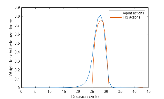
The fuzzy support system generates similar actions. However, it requires further optimizations to better match the agent actions.

Explanation Using Fuzzy Rule Inference

You can further explore the decision-making process of a FIS using its rule inference viewer. To do so, use the simFISWithInferenceViewer helper function. In this case, the fuzzy system drives the changes in the environment.

simFISWithInferenceViewer(env,fisout)

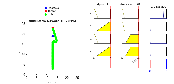
In each step, the rule inference process shows the fuzzification of the observation values, calculation of rule activation strengths, individual rule contributions in the output, and calculation of the final action value. Therefore, it shows an explainable visualization of the fuzzy rule applicability based on each observation of the environment.

Conclusion

You can further improve the performance of the fuzzy support system by using:

More test cases
Additional input MFs
Continuous MFs for smooth variations in the actions.

You can also intuitively update the fuzzy rule base to check possible variations of the current policy of the black-box model and, if possible, integrate the desired variations with existing black-box model.